39. Inventory Dynamics

39.1. Overview

In this lecture, we will study the time path of inventories for firms that follow so-called s-S inventory dynamics.

Such firms

1. wait until inventory falls below some level \(s\) and then

2. order sufficient quantities to bring their inventory back up to capacity \(S\).

These kinds of policies are common in practice and are also optimal in certain circumstances.

A review of early literature and some macroeconomic implications can be found in [Caplin, 1985].

Here, our main aim is to learn more about simulation, time series, and Markov dynamics.

While our Markov environment and many of the concepts we consider are related to those found in our lecture on finite Markov chains, the state space is a continuum in the current application.

Let’s start with some imports

from functools import partial
from typing import NamedTuple
import jax
import jax.numpy as jnp
from jax import random
import matplotlib.pyplot as plt
from sklearn.neighbors import KernelDensity

39.2. Sample paths

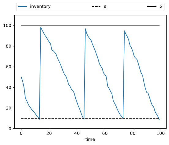
Consider a firm with inventory \(X_t\).

The firm waits until \(X_t \leq s\) and then restocks up to \(S\) units.

It faces stochastic demand \(\{ D_t \}\), which we assume is IID.

With notation \(a^+ := \max\{a, 0\}\), inventory dynamics can be written as

\[\begin{split} X_{t+1} = \begin{cases} ( S - D_{t+1})^+ & \quad \text{if } X_t \leq s \\ ( X_t - D_{t+1} )^+ & \quad \text{if } X_t > s \end{cases} \end{split}\]

In what follows, we will assume that each \(D_t\) is lognormal, so that

\[ D_t = \exp(\mu + \sigma Z_t) \]

where \(\mu\) and \(\sigma\) are parameters and \(\{Z_t\}\) is IID and standard normal.

Here’s a class that stores parameters and generates time paths for inventory.

class Firm(NamedTuple):
    s: int    # restock trigger level
    S: int    # capacity
    μ: float  # shock location parameter
    σ: float  # shock scale parameter

@partial(jax.jit, static_argnames="sim_length")
def sim_inventory_path(firm, x_init, key, sim_length):
    """
    Simulate an inventory path of length sim_length from a single key.

    A fresh shock is generated each period by folding the period index
    into key, so callers pass one key per path rather than a whole array.

    Args:
        firm: Firm object
        x_init: Initial inventory level
        key: A single JAX random key
        sim_length: Number of periods to simulate

    Returns:
        Array of inventory levels [X_0, X_1, ..., X_{sim_length-1}]
    """

    def update(t, X):
        x = X[t - 1]
        Z = random.normal(random.fold_in(key, t))   # fresh shock for period t
        D = jnp.exp(firm.μ + firm.σ * Z)
        x_new = jnp.where(
            x <= firm.s,
            jnp.maximum(firm.S - D, 0.0),   # restock to S, then meet demand
            jnp.maximum(x - D, 0.0),        # just meet demand
        )
        return X.at[t].set(x_new)

    X = jnp.zeros(sim_length).at[0].set(x_init)
    return jax.lax.fori_loop(1, sim_length, update, X)

Note

Writing X.at[t].set(x_new) returns a new array rather than mutating X in place, in keeping with JAX’s functional style. This is not as wasteful as it looks: inside a jax.jit-compiled function the XLA compiler sees that the old array is no longer needed and performs the update in place, so no fresh array is allocated each period.

firm = Firm(s=10, S=100, μ=1.0, σ=0.5)

sim_length = 100
x_init = 50
X = sim_inventory_path(firm, x_init, random.key(21), sim_length)

Let’s run a first simulation, of a single path:

s, S = firm.s, firm.S

fig, ax = plt.subplots()
bbox = (0.0, 1.02, 1.0, 0.102)
legend_args = {"ncol": 3, "bbox_to_anchor": bbox, "loc": 3, "mode": "expand"}

ax.plot(X, label="inventory")
ax.plot(jnp.full(sim_length, s), "k--", label="$s$")
ax.plot(jnp.full(sim_length, S), "k-", label="$S$")
ax.set_ylim(0, S + 10)
ax.set_xlabel("time")
ax.legend(**legend_args)

plt.show()

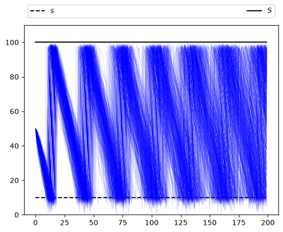
Now let’s simulate multiple paths in order to build a more complete picture of the probabilities of different outcomes:

sim_length = 200
fig, ax = plt.subplots()

ax.plot(jnp.full(sim_length, s), "k--", label="$s$")
ax.plot(jnp.full(sim_length, S), "k-", label="$S$")
ax.set_ylim(0, S + 10)
ax.legend(**legend_args)

for i in range(400):
    X = sim_inventory_path(firm, x_init, random.key(i), sim_length)
    ax.plot(X, "b", alpha=0.2, lw=0.5)

plt.show()

39.3. Marginal distributions

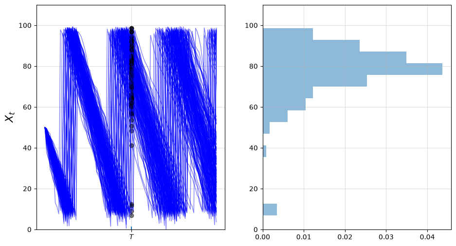
Now let’s look at the marginal distribution \(\psi_T\) of \(X_T\) for some fixed \(T\).

We will do this by generating many draws of \(X_T\) given initial condition \(X_0\).

With these draws of \(X_T\) we can build up a picture of its distribution \(\psi_T\).

Here’s one visualization, with \(T=50\).

T = 50
M = 200  # Number of draws

ymin, ymax = 0, S + 10

fig, axes = plt.subplots(1, 2, figsize=(11, 6))

for ax in axes:
    ax.grid(alpha=0.4)

ax = axes[0]

ax.set_ylim(ymin, ymax)
ax.set_ylabel("$X_t$", fontsize=16)
ax.vlines((T,), -1.5, 1.5)

ax.set_xticks((T,))
ax.set_xticklabels((r"$T$",))

sample = []
for m in range(M):
    X = sim_inventory_path(firm, x_init, random.key(m), 2 * T)
    ax.plot(X, "b-", lw=1, alpha=0.5)
    ax.plot((T,), (X[T],), "ko", alpha=0.5)
    sample.append(X[T])

axes[1].set_ylim(ymin, ymax)

axes[1].hist(
    sample,
    bins=16,
    density=True,
    orientation="horizontal",
    histtype="bar",
    alpha=0.5,
)

plt.show()

We can build up a clearer picture by drawing more samples

T = 50
M = 50_000

fig, ax = plt.subplots()

# Draw all M paths at once by vectorizing over one key per path
keys = random.split(random.key(0), M)
paths = jax.vmap(
    sim_inventory_path, in_axes=(None, None, 0, None)
)(firm, x_init, keys, T + 1)
sample = paths[:, T]

ax.hist(sample, bins=36, density=True, histtype="bar", alpha=0.75)

plt.show()

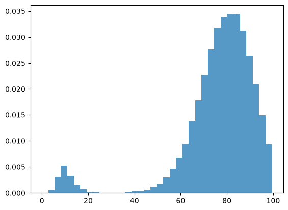
Note that the distribution is bimodal

• Most firms have restocked twice but a few have restocked only once (see figure with paths above).

• Firms in the second category have lower inventory.

We can also approximate the distribution using a kernel density estimator.

Kernel density estimators can be thought of as smoothed histograms.

They are preferable to histograms when the distribution being estimated is likely to be smooth.

We will use a kernel density estimator from scikit-learn

def plot_kde(sample, ax, label=""):
    xmin, xmax = 0.9 * sample.min(), 1.1 * sample.max()
    xgrid = jnp.linspace(xmin, xmax, 200)
    kde = KernelDensity(kernel="gaussian").fit(sample[:, None])
    log_dens = kde.score_samples(xgrid[:, None])

    ax.plot(xgrid, jnp.exp(log_dens), label=label)

fig, ax = plt.subplots()
plot_kde(sample, ax)
plt.show()

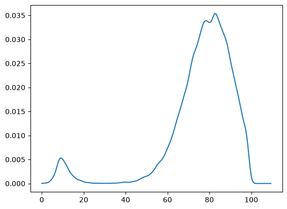
The allocation of probability density is similar to what was shown by the histogram just above.

39.4. Exercises

Exercise 39.1

This model is asymptotically stationary, with a unique stationary distribution.

(See the discussion of stationarity in our lecture on AR(1) processes for background — the fundamental concepts are the same.)

In particular, the sequence of marginal distributions \(\{\psi_t\}\) is converging to a unique limiting distribution that does not depend on initial conditions.

Although we will not prove this here, we can investigate it using simulation.

Your task is to generate and plot the sequence \(\{\psi_t\}\) at times \(t = 10, 50, 250, 500, 750\) based on the discussion above.

(The kernel density estimator is probably the best way to present each distribution.)

You should see convergence, in the sense that differences between successive distributions are getting smaller.

Try different initial conditions to verify that, in the long run, the distribution is invariant across initial conditions.

Solution

Below is one possible solution:

The computations involve a lot of CPU cycles so we have tried to write the code efficiently using jax.jit and jax.vmap to run on CPU/GPU.

@jax.jit
def simulate_firm_forward(firm, x_init, key, num_periods):
    """
    Simulate a single firm num_periods steps forward and return its
    final inventory level. A fresh shock is drawn each period from key.
    """

    def update(t, x):
        Z = random.normal(random.fold_in(key, t))
        D = jnp.exp(firm.μ + firm.σ * Z)
        return jnp.where(
            x <= firm.s,
            jnp.maximum(firm.S - D, 0.0),
            jnp.maximum(x - D, 0.0),
        )

    return jax.lax.fori_loop(0, num_periods, update, x_init * 1.0)


# Vectorize over firms: each has its own initial level and its own key
simulate_firms_forward = jax.vmap(
    simulate_firm_forward, in_axes=(None, 0, 0, None)
)

def shift_firms_forward(firm, current_inventory_levels, num_periods, key):
    """
    Shift multiple firms forward by num_periods using JAX vectorization.
    Returns:
        Array of new inventory levels after num_periods
    """

    # Generate one independent random key per firm
    num_firms = len(current_inventory_levels)
    firm_keys = random.split(key, num_firms)
    # Run simulation for all firms in parallel
    new_inventory_levels = simulate_firms_forward(
        firm, current_inventory_levels, firm_keys, num_periods
    )

    return new_inventory_levels

x_init = 50
num_firms = 50_000

sample_dates = 0, 10, 50, 250, 500, 750

first_diffs = jnp.diff(jnp.array(sample_dates))

fig, ax = plt.subplots()

X = jnp.full(num_firms, x_init)

current_date = 0
for d in first_diffs:
    X = shift_firms_forward(firm, X, d, random.key(current_date + 1))
    current_date += d
    plot_kde(X, ax, label=f"t = {current_date}")

ax.set_xlabel("inventory")
ax.set_ylabel("probability")
ax.legend()
plt.show()

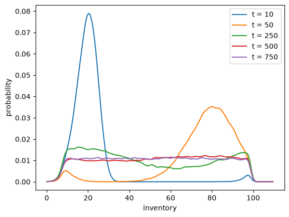
Notice that by \(t=500\) or \(t=750\) the densities are barely changing.

We have reached a reasonable approximation of the stationary density.

You can convince yourself that initial conditions don’t matter by testing a few of them.

For example, try rerunning the code above with all firms starting at \(X_0 = 20\) or \(X_0 = 80\).

Exercise 39.2

Using simulation, calculate the probability that firms that start with \(X_0 = 70\) need to order twice or more in the first 50 periods.

You will need a large sample size to get an accurate reading.

Solution

Here is one solution.

Again, the computations are relatively intensive so we have written a specialized JAX-jitted function and using jax.vmap to use parallelization across firms.

Note the time the routine takes to run, as well as the output.

@jax.jit
def simulate_firm_restocks(firm, x_init, key, num_periods):
    """
    Simulate a single firm for num_periods and report whether it
    restocked more than once. A fresh shock is drawn each period from key.

    Returns:
        1 if the firm restocks > 1 times, 0 otherwise
    """

    def update(t, carry):
        x, restock_count = carry
        Z = random.normal(random.fold_in(key, t))
        D = jnp.exp(firm.μ + firm.σ * Z)
        restock = x <= firm.s
        x_new = jnp.where(
            restock,
            jnp.maximum(firm.S - D, 0.0),
            jnp.maximum(x - D, 0.0),
        )
        return x_new, restock_count + restock

    # Carry the inventory level and a running restock count
    _, total_restocks = jax.lax.fori_loop(
        0, num_periods, update, (x_init * 1.0, 0)
    )
    return (total_restocks > 1).astype(jnp.int32)


# Vectorize the simulation across all firms (one key each)
simulate_firms_restocks = jax.vmap(
    simulate_firm_restocks, in_axes=(None, None, 0, None)
)

def compute_freq(
    firm, x_init=70, sim_length=50, num_firms=1_000_000, key=random.key(2)
):
    """
    Compute the frequency of firms that restock 2 or more times using JAX.

    Args:
        firm: Firm dataclass
        x_init: Initial inventory level for all firms
        sim_length: Length of simulation for each firm
        num_firms: Number of firms to simulate
        key: JAX random key

    Returns:
        Fraction of firms that restock 2 or more times
    """
    # Generate one independent random key per firm
    firm_keys = random.split(key, num_firms)
    # Run simulation for all firms
    restock_indicators = simulate_firms_restocks(
        firm, x_init, firm_keys, sim_length
    )
    # Compute frequency (fraction of firms that restocked > 1 times)
    frequency = jnp.mean(restock_indicators)
    return frequency

%%time

freq = compute_freq(firm)
print(f"Frequency of at least two stock outs = {freq}")

Frequency of at least two stock outs = 0.44668900966644287
CPU times: user 1.07 s, sys: 33.1 ms, total: 1.1 s
Wall time: 770 ms