89. Adaptive Learning and Escape Dynamics#
89.1. Overview#
This lecture is the culmination of the Phillips curve tradeoffs suite.
It follows chapter 8 of [Sargent, 1999], the most ambitious chapter of the book.
In Self-Confirming Equilibria a government held fixed beliefs about the Phillips curve — beliefs that were confirmed by the data those beliefs generated.
Here we make the government a real-time econometrician.
Each period it
re-estimates its Phillips curve by recursive least squares from the data seen so far, and
sets inflation at the first-period recommendation of the Phelps problem for its current estimate.
We ask whether such an adaptive government converges to a self-confirming equilibrium.
The answer depends on a single parameter — the gain that governs how fast old data are discounted:
With a decreasing gain that implements least squares, the mean dynamics pull the economy to a self-confirming equilibrium, and we get nothing new: the system is stuck near the Nash outcome.
With a constant gain, agents discount past data, convergence is arrested, and new outcomes emerge. The system recurrently escapes the self-confirming equilibrium toward the Ramsey (zero-inflation) outcome — spontaneous stabilizations that resemble the arrival of Volcker.
These escapes are the heart of the vindication of econometric policy evaluation story from The Rise and Fall of U.S. Inflation: an adaptive government, learning a Solow-Tobin distributed-lag version of the natural-rate hypothesis, is led by chance observations to stabilize inflation.
This lecture replicates, analyzes, and reinterprets simulations like those of Christopher Sims and Heetaik Chung [Chung, 1990, Sims, 1988].
Here we study the escapes by simulation; Escaping Nash Inflation then characterizes them analytically as a second, deterministic ODE, and Priors, Escapes, and Learning Cycles asks how the government’s prior about coefficient drift reshapes both forces.
Let’s import what we need:
import matplotlib.pyplot as plt
import numpy as np
from scipy.linalg import solve_discrete_are
89.2. A primer on recursive algorithms#
This section is a self-contained primer.
It develops the two analytical objects — mean dynamics and escape routes — that organize everything that follows, and it explains the sense in which one and the same recursion can be read either as an algorithm for computing a self-confirming equilibrium or as a model of a government adapting in real time.
The material is technical, and readers who want the punchline can skip to the simulations below and refer back as needed.
89.2.1. Beliefs, moment conditions, and self-confirming equilibria#
A self-confirming equilibrium under the classical identification is pinned down by the government’s beliefs about some population moments and the regression coefficients they imply.
Under the classical identification these beliefs are measured by the triple \((\gamma, \, E X_{C} X_{C}', \, E U X_{C})\), where \(\gamma\) is the vector of Phillips-curve coefficients.
In the adaptive models of this lecture the time-\(t\) values of these objects are among the economy’s state variables; they disappear as state variables in a self-confirming equilibrium only because there they are constants.
A self-confirming equilibrium under the classical identification satisfies the moment conditions
where the mathematical expectation is taken with respect to a distribution of \((U_t, X_{Ct})\) that depends on \(\gamma\) through the solution \(h(\gamma)\) of the Phelps problem.
Self-reference surfaces precisely in this dependence of the distribution on \(\gamma\): the government’s beliefs shape its policy, which shapes the data on which the beliefs are then checked.
The first line of (89.1) is the least squares normal equations for \(\gamma\), pre-multiplied by the inverse second-moment matrix; the second line defines \(R_{XC}\) as the second-moment matrix of the regressors.
It is convenient to assemble all the unknowns into a single vector
where \(\operatorname{col}(R_{XC})\) stacks the columns of \(R_{XC}\).
The moment conditions (89.1) then take the compact form
where \(\zeta\) is a random vector and the expectation is over its distribution (which, again, depends on \(\phi\)).
A self-confirming equilibrium is a set of beliefs \(\phi_f\) that is a zero of \(b\),
The rest of this section describes recursive algorithms for finding such a zero, and a change of perspective that converts each computational algorithm into a model of real-time adaptation.
89.2.2. Iteration#
The simplest algorithm computes a sequence \(\{\phi_k\}\) of estimates from
where the distribution used to evaluate the expectation defining \(b(\phi_k)\) in (89.3) is itself evaluated at the current estimate \(\phi_k\), and \(a > 0\) is a step size.
This is the relaxation algorithm used to compute self-confirming equilibria in Self-Confirming Equilibria.
Each step requires evaluating the mathematical expectation \(b(\phi) = E[F(\phi, \zeta)]\) — which is exactly why we needed the moment (Lyapunov) formulas there.
89.2.3. Stochastic approximation#
A random version of (89.5) is obtained by replacing the mean \(b(\phi_n)\) by a single random draw \(F(\phi_n, \zeta_n)\) and letting the step size do the averaging:
To study the limiting behavior of (89.6), define artificial time
form the sampled process \(\phi(t_n) = \phi_n\), and interpolate (typically piecewise-linearly) to obtain a continuous-time process \(\phi^o(t)\).
One then approximates \(\phi^o(t)\) by a continuous-time process as \(n \to \infty\) and uses it to characterize the tail of the original sequence.
Different rates of decrease of the gain sequence \(\{a_n\}\) produce different approximating processes, because they change the mapping (89.7) from real time \(n\) to artificial time \(t_n\).
Note
Recursive stochastic approximation originates with [Robbins and Monro, 1951], who devised (89.6) to find the root of a regression function observed with noise, and with [Kiefer and Wolfowitz, 1952], who adapted it to find the maximum of a regression function (the “K-W” algorithms referred to below). The “ODE method” for analyzing such recursions — approximating the interpolated process by the solution of a differential equation — is due to [Ljung, 1977]; book-length treatments are [Benveniste et al., 1990] and [Kushner and Yin, 2003]. Its use to study learning in self-referential macroeconomic models is developed by [Marcet and Sargent, 1989] and, comprehensively, by [Evans and Honkapohja, 2001].
89.2.4. Mean dynamics#
The classic stochastic approximation algorithms of [Kushner and Clark, 1978] and [Ljung, 1977] set the gain to decrease like \(a_n \sim 1/n\) (at least for \(t \geq N\) for some \(N > 0\)).
This permits strong statements about the almost sure convergence of (89.6) to a zero of \(b(\phi)\).
For \(a_n \sim 1/n\), as \(n \to \infty\) the interpolated process \(\phi^o(t)\) approaches the solution of the ordinary differential equation
which we call the mean dynamics — the vector generalization of the scalar least-squares-learning ODE derived in the appendix of The Credibility Problem.
A law of large numbers makes the random term in the continuous-time approximation vanish fast enough that the mean dynamics (89.8) describe the tail behavior of the stochastic process (89.6).
Consequently:
if the algorithm converges (almost surely), it converges to a zero of the mean dynamics, \(b(\phi) = 0\) — a self-confirming equilibrium; and
the ODE (89.8) carries the information about local and global stability of the algorithm.
Local stability is governed by the eigenvalues of the Jacobian of \(b\) at a rest point: if all eigenvalues have negative real parts the rest point is locally stable, and, under conditions on the gain, the eigenvalue of largest real part governs the rate of convergence (the usual \(\sqrt{T}\) rate requires that eigenvalue to be below \(-\tfrac12\)).
We will see below that for the classical model at our parameters this eigenvalue sits exactly at the \(-\tfrac12\) boundary, so convergence is marginal — a fact that turns out to matter for how readily the system escapes.
Note
[Brock and Hommes, 1997] build models whose global behavior is driven by stable mean dynamics far from rational expectations equilibria together with local instability of adaptation near them — a complementary mechanism for generating endogenous fluctuations from learning.
89.2.5. Constant gain and convergence in distribution#
We are equally interested in versions of (89.6) with a constant gain \(a_n = \epsilon > 0\) for all \(n\).
Limit theorems for constant-gain algorithms use a weaker notion of convergence — convergence in distribution — than the almost-sure convergence available when \(a_n \sim 1/n\).
They concern small-noise limits, taken as \(\epsilon \to 0\) and \(n\epsilon \to +\infty\) simultaneously.
Again using artificial time (89.7), form the family of processes
interpolate to obtain \(\phi^\epsilon(t)\), and study its small-\(\epsilon\) limit.
Dupuis and Kushner, [Kushner and Yin, 2003], and others verified conditions under which, as \(\epsilon \to 0\) and \(\epsilon n \to \infty\), the process \(\phi_n^\epsilon\) converges in distribution to the zeros of the same mean dynamics (89.8); the restrictions on the mean dynamics needed for convergence match those from the classic \(a_n \sim 1/n\) theory.
Unlike the decreasing-gain algorithm, a constant-gain algorithm does not settle down: \((\gamma, R_{XC})\) converges to a stationary stochastic process, perpetually fluctuating around — and occasionally far from — the self-confirming equilibrium.
89.2.6. Escape routes and the theory of large deviations#
The feature of the constant-gain apparatus that matters most for this lecture is not convergence toward \(\phi_f\) but the excursions away from it.
We are as interested in movements away from a self-confirming equilibrium as in those toward one, because the recurrent stabilizations in the simulations are precisely such excursions.
The theory of large deviations characterizes these excursions through three objects.
First, the log moment generating function of (an averaged version of) the innovation process \(F(\phi_n, \zeta_n)\): for a vector \(\theta\) conformable to \(F\),
where the expectation is over the distribution of \(\zeta\).
Note
Equation (89.10) is a heuristic shorthand. The object that actually enters the theory is a time-averaged limit; [Dupuis and Kushner, 1987] and [Kushner and Yin, 2003] assume that for each \(\delta > 0\) the following limit exists uniformly in \(\phi_i, \alpha_i\) on any compact set: $\( \sum_{i=0}^{T/\delta - 1} \delta\, H(\alpha_i, \phi_i) = \lim_{N \to \infty} \frac{\delta}{N} \log E \exp \sum_{i=0}^{T/\delta - 1} \alpha_i' \sum_{j=iN}^{iN+N-1} F(\phi_i, \zeta_j) . \)\( The inner sum averages the innovations over a block of length \)N$; the double limit lets us treat serially dependent innovations.
Second, the Legendre transform of \(H\), which plays the role of a rate function:
Third, the action functional, which measures the “cost” of a candidate escape path \(\phi(\cdot)\):
Dupuis and Kushner turn the search for the most likely escape into a deterministic control problem.
Let \(D\) be a compact set containing \(\phi_f\), with boundary \(\partial D\), and let \(C[0,T]\) be the continuous functions on \([0,T]\).
The escape route is the path \(\tilde\phi(\cdot)\) that solves
Assuming the minimizer \(\tilde\phi(\cdot)\) is unique, and letting \(t_D^\epsilon\) be the first time the constant-gain process \(\phi^\epsilon(t)\) leaves \(D\), [Dupuis and Kushner, 1987] show that for every \(\delta > 0\)
In words: conditional on escaping the set \(D\), the system leaves it near the terminal point of the least-action path — so the escape has a deterministic direction and shape, even though it is triggered by chance.
This is the sense in which the escapes below, though they require no large shock, “seem purposeful”: they follow the least-action route dictated by (89.13).
A crucial contrast with the mean dynamics: the mean dynamics (89.8) do not depend on the noise around them, whereas the escape routes do — the noise not only adds random fluctuations around (89.8), it also carves out this second family of paths.
Note
The mathematical foundations are the large-deviation theory for randomly perturbed dynamical systems of [Freidlin and Wentzell, 1998] (especially their chapter 4), specialized to stochastic approximation by [Dupuis and Kushner, 1987] and [Dupuis and Kushner, 1989]; a weak-convergence treatment is [Dupuis and Ellis, 1997].
89.2.7. A tractable action functional#
The escape-route calculation promises cheap information about central tendencies of the algorithm, but the action functional (89.12) is generally hard to compute.
An important special case simplifies it dramatically.
Suppose the innovation is additive and Gaussian,
where \(\zeta_n\) is stationary and Gaussian but not necessarily serially uncorrelated, and define \(R = \sum_j E\, \zeta_t \zeta_{t-j}'\).
Then the action functional takes the quadratic form
where \((\cdot)^{+}\) is the Moore-Penrose generalized inverse (used to handle possible stochastic singularity of \(\sigma R \sigma'\)).
The weight \(h(s)\) depends on the gain: \(h(s) = \exp(s)\) when \(\gamma = 1\) in \(a_n = a_0 / n^\gamma\), and \(h(s) = 1\) when \(\gamma < 1\).
Read (89.15) as a cost that penalizes departures of the realized drift \(\tfrac{d}{ds}\phi\) from the mean drift \(b(\phi)\), weighting each direction by the inverse of the local noise covariance \(\sigma R \sigma'\).
The least-action escape therefore threads the beliefs through regions where the mean dynamics are weak and the noise is informative — which, in our model, is the direction of the induction hypothesis.
Note
This quadratic action functional is precisely the object minimized in [Cho et al., 2002], the published treatment of the model of this lecture. They solve the control problem (89.13) for the Nash self-confirming equilibrium and show, analytically, that the least-action escape drives the sum of weights on inflation toward the value that activates the induction hypothesis — that is, toward the Ramsey outcome. [Sargent and Williams, 2005] study how the government’s prior (equivalently, the covariance structure of the gain algorithm, our \(P_0\) and forgetting factor) reshapes the escape, and [Kasa, 2004] applies the same large-deviation machinery to recurrent currency crises.
89.2.8. From computation to adaptation#
The preceding recursions were introduced as algorithms to approximate a self-confirming equilibrium.
The same mathematics tells us what happens when we instead modify our self-confirming-equilibrium models to incorporate real-time adaptation — simply by reading \(\phi_n\) as the government’s time-\(n\) beliefs rather than as the \(n\)-th iterate of a solver.
Two facts organize everything below:
gain sequences that implement least squares (decreasing like \(1/t\)) make the mean dynamics pull the economy toward self-confirming equilibria; while
gain sequences that fall off more slowly — in the limit, constant gains that discount the past — arrest that pull and increase the frequency with which the escape dynamics influence outcomes.
Note
A brief intellectual history. [Lucas and Prescott, 1971] dismissed iterating on the moment conditions (89.4) as a computational strategy, but [Townsend, 1983] used it. [Woodford, 1990] and [Marcet and Sargent, 1989] used the mean dynamics (89.8) to establish conditions for the convergence of least squares learning to rational expectations in models with self-reference, both requiring continuity of \(b(\phi)\). In-Koo Cho studied problems with discontinuous \(b(\phi)\) inherited from discontinuous decision rules (trigger strategies in credibility and search problems); to make least squares learning approach rational expectations he used gains satisfying \(\tfrac{1}{\log n} < a_n < \tfrac{1}{\sqrt n}\), which yield a diffusion approximation to (89.6) that promotes enough experimentation to discover an equilibrium. [Kandori et al., 1993] use related mathematics to select long-run equilibria in games via mutation, and Roger Myerson applied an escape-route calculation to a voting problem. The modern synthesis of these learning methods is [Evans and Honkapohja, 2001].
89.3. The adaptive model#
We now build the classical adaptive model.
89.3.1. Government beliefs and behavior#
The government believes in a distributed-lag Phillips curve
Arriving at time \(t\) with an estimate \(\gamma_{t-1}\), it sets the systematic part of inflation by solving the Phelps problem as if \(\gamma_{t-1}\) will govern the Phillips curve forever:
It then updates its beliefs by recursive least squares (RLS):
where \(\{g_t\}\) is the gain sequence.
Least squares sets \(g_t = 1/t\); a constant-gain algorithm sets \(g_t = g_0 > 0\) and discounts past observations, which is sensible if the government suspects the Phillips curve wanders over time.
The public is assumed to know the government’s rule, so its inflation forecast is \(x_t = h(\gamma_{t-1}) X_{t-1}\), the systematic part of (89.17).
Unemployment is generated by the actual Phillips curve of Self-Confirming Equilibria with \(\rho_1 = \rho_2 = 0\):
89.3.2. The Phelps problem with lags#
Given a belief \(\gamma\), the decision rule \(h(\gamma)\) solves an LQ control problem.
Write the believed Phillips curve as \(U_t = \gamma_0 y_t + c' s_t\), where \(\gamma_0\) is the coefficient on current inflation and \(c\) collects the coefficients on the state \(s_t = X_{t-1}\).
The government minimizes \(E\sum_t \delta^t (U_t^2 + y_t^2)\), so the per-period loss is \(s_t' (cc') s_t + (\gamma_0^2 + 1) y_t^2 + 2\gamma_0\, y_t\, c' s_t\), and the state evolves as \(s_{t+1} = A s_t + B y_t\) with
We solve the discounted LQ problem with scipy’s discrete algebraic Riccati equation.
class AdaptivePhillips:
    """
    Classical adaptive Phillips curve model: the government re-estimates a
    distributed-lag Phillips curve by recursive least squares and each period
    acts on the first-period recommendation of the Phelps problem.
    """

    def __init__(self, θ=1.0, U_star=5.0, σ1=0.3, σ2=0.3, δ=0.98):
        self.θ, self.U_star, self.σ1, self.σ2, self.δ = θ, U_star, σ1, σ2, δ

        # classical self-confirming belief: U = -θ y + (θ²+1)U*
        self.γ_sce = np.array([-θ, 0.0, 0.0, 0.0, 0.0, (θ**2 + 1) * U_star])

        # self-confirming moment matrix M = E[X_C X_C'] and residual variance
        self.M = self._sce_moments()
        self.σC2 = σ1**2                       # var(U | X_C) at the SCE

    def _sce_moments(self):
        "E[X_C X_C'] at the serially-uncorrelated classical SCE."
        θ, σ1, σ2 = self.θ, self.σ1, self.σ2
        μU, μy = self.U_star, self.θ * self.U_star
        Σ = {('U', 'U'): θ**2 * σ2**2 + σ1**2, ('y', 'y'): σ2**2,
             ('U', 'y'): -θ * σ2**2, ('y', 'U'): -θ * σ2**2}
        # regressors: (time, type) for [y_t, U_{t-1}, U_{t-2}, y_{t-1}, y_{t-2}, 1]
        regs = [(0, 'y'), (1, 'U'), (2, 'U'), (1, 'y'), (2, 'y'), (None, 'c')]
        mean = {'U': μU, 'y': μy, 'c': 1.0}
        M = np.zeros((6, 6))
        for i, (ti, tyi) in enumerate(regs):
            for j, (tj, tyj) in enumerate(regs):
                if tyi == 'c' or tyj == 'c' or ti != tj:
                    M[i, j] = mean[tyi] * mean[tyj]
                else:
                    M[i, j] = Σ[(tyi, tyj)] + mean[tyi] * mean[tyj]
        return M

    def phelps_h(self, γ):
        "Government decision rule ŷ_t = h(γ)·X_{t-1} for belief γ."
        δ, γ0, c = self.δ, γ[0], γ[1:]
        R = np.outer(c, c)
        Q = np.array([[γ0**2 + 1.0]])
        N = (γ0 * c).reshape(1, -1)
        A = np.zeros((5, 5)); B = np.zeros((5, 1))
        A[0, :] = c; B[0, 0] = γ0          # U_t
        A[1, 0] = 1.0                       # U_{t-1}
        B[2, 0] = 1.0                       # y_t
        A[3, 2] = 1.0                       # y_{t-1}
        A[4, 4] = 1.0                       # constant
        sb = np.sqrt(δ)
        Ad, Bd = sb * A, sb * B
        P = solve_discrete_are(Ad, Bd, R, Q, s=sb * N.T)
        F = np.linalg.solve(Q + Bd.T @ P @ Bd, Bd.T @ P @ Ad + N)
        return -F.ravel()
We use the Kalman-filter implementation of RLS from Appendix A of [Sargent, 1999].
A forgetting factor \(\lambda \in (0, 1]\) maps to the gain: \(\lambda = 1\) gives least squares (\(g_t \to 1/t\)), while \(\lambda < 1\) gives a constant gain \(g_0 = 1 - \lambda\).
The prior is initialized as if the government had already seen \(T\) periods of self-confirming-equilibrium data, through \(P_0 = (\sigma_C^2 / T)\, M^{-1}\); larger \(T\) means a tighter prior.
def simulate(model, λ, T_prior, n=1000, seed=0):
    "Simulate the adaptive system. λ=1 is least squares; λ<1 is constant gain."
    rng = np.random.default_rng(seed)
    θ, U_star, σ1, σ2 = model.θ, model.U_star, model.σ1, model.σ2

    γ = model.γ_sce.copy()
    P = (model.σC2 / T_prior) * np.linalg.inv(model.M)
    R2 = model.σC2
    g0 = 1 - λ

    U1 = U2 = U_star
    y1 = y2 = θ * U_star
    y_path, U_path, sumweights, constant = (np.empty(n) for _ in range(4))

    for t in range(n):
        h = model.phelps_h(γ)
        X_lag = np.array([U1, U2, y1, y2, 1.0])
        yhat = h @ X_lag

        v2, v1 = σ2 * rng.standard_normal(), σ1 * rng.standard_normal()
        y = yhat + v2
        U = U_star - θ * (y - yhat) + v1

        φ = np.array([y, U1, U2, y1, y2, 1.0])           # X_C,t
        denom = R2 + φ @ P @ φ
        gain = P @ φ / denom
        γ = γ + gain * (U - γ @ φ)
        R1 = (g0 / (1 - g0)) * P if λ < 1 else 0.0        # constant vs decreasing
        P = P - np.outer(P @ φ, φ @ P) / denom + R1

        y_path[t], U_path[t] = y, U
        sumweights[t] = γ[0] + γ[3] + γ[4]               # weights on current+lagged y
        constant[t] = γ[5]
        U2, U1 = U1, U
        y2, y1 = y1, y

    return dict(y=y_path, U=U_path, sumweights=sumweights, constant=constant)
model = AdaptivePhillips()
h_sce = model.phelps_h(model.γ_sce)
print("decision rule at the self-confirming belief:")
print(f"  h(γ_sce) = {np.round(h_sce, 3)}  (a constant rule of "
      f"{h_sce[-1]:.1f} = Nash inflation)")
decision rule at the self-confirming belief:
  h(γ_sce) = [-0. -0. -0. -0.  5.]  (a constant rule of 5.0 = Nash inflation)
At the self-confirming belief the Phelps rule is a constant equal to the Nash inflation rate, and the beliefs reproduce themselves — the adaptive system’s rest point is the self-confirming equilibrium of Self-Confirming Equilibria.
89.4. Least squares learning converges#
We follow [Sargent, 1999] in setting the true data-generating parameters to the classical example at the end of Self-Confirming Equilibria: \(U^* = 5\), \(\theta = 1\), \(\sigma_1 = \sigma_2 = 0.3\), \(\rho_1 = \rho_2 = 0\), \(\delta = 0.98\).
The classical self-confirming equilibrium has serially uncorrelated \((U, y)\) fluctuating around means \((5, 5)\).
First, least squares (a decreasing gain).
ls = simulate(model, λ=1.0, T_prior=5000, n=1000, seed=1)

fig, ax = plt.subplots(figsize=(9, 4.5))
ax.plot(ls['y'], lw=0.8)
ax.axhline(5, color='k', ls='--', lw=1, label='self-confirming (Nash)')
ax.axhline(0, color='C2', ls=':', lw=1, label='Ramsey')
ax.set_xlabel('$t$')
ax.set_ylabel('inflation $y_t$')
ax.set_title('Figure 8.1: classical adaptive model, least squares')
ax.legend()
plt.show()
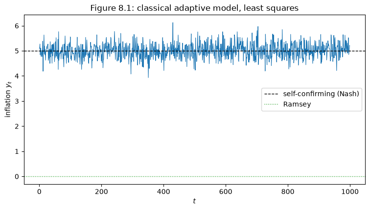
Under least squares the mean dynamics dominate: inflation hugs the self-confirming value of 5, and the simulation looks like a draw from the self-confirming equilibrium itself.
We get nothing new — the government is stuck near the Nash outcome.
89.5. Constant gain and escape dynamics#
Now give the government a constant gain, \(\lambda = 0.975\), so it discounts past data.
cg = simulate(model, λ=0.975, T_prior=300, n=1000, seed=1)

fig, ax = plt.subplots(figsize=(9, 4.5))
ax.plot(cg['y'], lw=0.8)
ax.axhline(5, color='k', ls='--', lw=1, label='self-confirming (Nash)')
ax.axhline(0, color='C2', ls=':', lw=1, label='Ramsey')
ax.set_xlabel('$t$')
ax.set_ylabel('inflation $y_t$')
ax.set_title('Figure 8.2: classical adaptive model, constant gain '
             r'($\lambda = 0.975$)')
ax.legend()
plt.show()
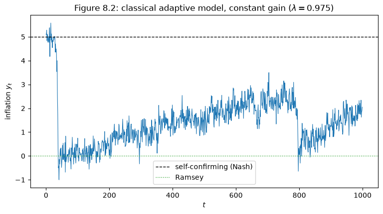
The picture is completely different.
Inflation starts near the self-confirming value of 5, then drops almost to zero and stays there for a long time, before slowly heading back toward 5 only to be propelled toward zero again.
The mean dynamics that pull the system toward the self-confirming equilibrium are opposed by a recurrent force that sends inflation close to the Ramsey outcome.
Crucially, no large shocks trigger these stabilizations: they are an endogenous feature of the constant-gain learning dynamics.
print(f"constant-gain inflation: mean {cg['y'].mean():.2f}, "
      f"fraction of periods near Ramsey (y<2): {(cg['y'] < 2).mean():.0%}")
constant-gain inflation: mean 1.41, fraction of periods near Ramsey (y<2): 77%
89.6. The escape route and the induction hypothesis#
Why does the system escape toward Ramsey rather than in some other direction?
The answer is the induction hypothesis of Adaptive Expectations and the Phelps Problem: when the sum of the weights on current and lagged inflation in the estimated Phillips curve approaches zero, the Phelps problem advises the government to reduce inflation.
Let’s plot inflation together with that sum of weights.
fig, axes = plt.subplots(2, 1, figsize=(9, 7), sharex=True)

axes[0].plot(cg['y'], lw=0.8)
axes[0].axhline(0, color='C2', ls=':', lw=1)
axes[0].set_ylabel('inflation $y_t$')

axes[1].plot(cg['sumweights'], lw=0.8, color='C1')
axes[1].axhline(-1, color='k', ls='--', lw=1, label='self-confirming value')
axes[1].axhline(0, color='C3', ls=':', lw=1, label='induction hypothesis')
axes[1].set_xlabel('$t$')
axes[1].set_ylabel('sum of weights on $y$')
axes[1].legend()

fig.suptitle('Escape route: stabilizations coincide with the sum of '
             'weights rising toward zero')
plt.tight_layout()
plt.show()
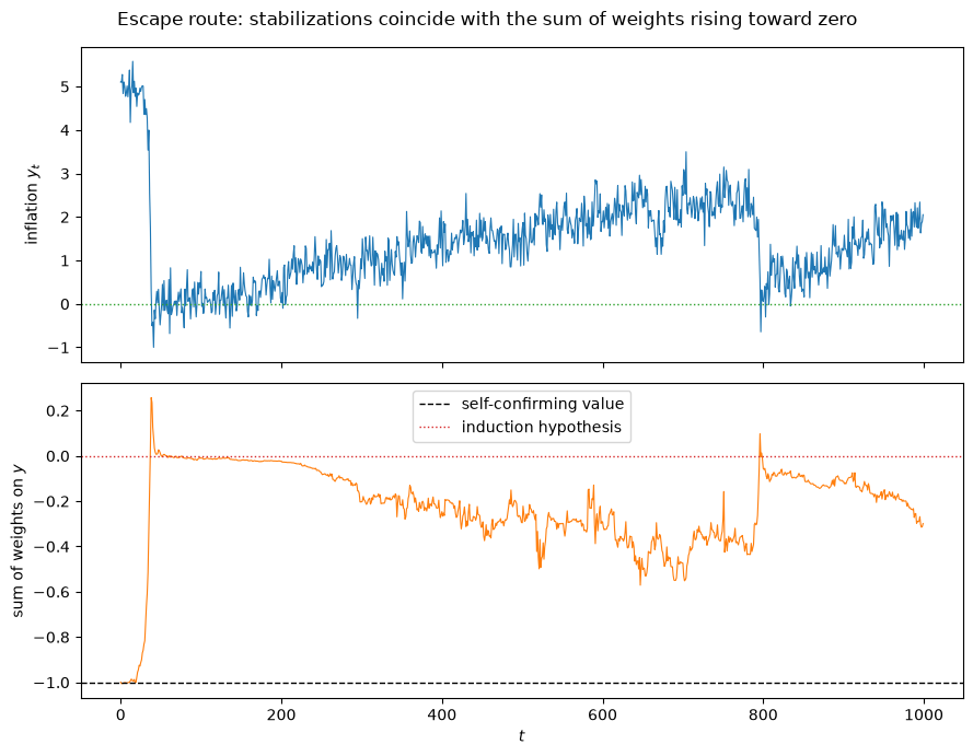
Every stabilization coincides with the sum of weights jumping from its self-confirming value of \(-1\) toward zero.
When it reaches zero, the induction hypothesis is (temporarily) satisfied, the Phelps problem calls for near-Ramsey inflation, and the resulting data briefly reinforce the induction hypothesis — a situation that is not self-confirming in the technical sense but is nonetheless self-reinforcing.
We can see the escape route directly by plotting the joint path of the constant and the sum of weights in the estimated Phillips curve.
fig, ax = plt.subplots(figsize=(8, 6))
sc = ax.scatter(cg['constant'], cg['sumweights'], c=np.arange(len(cg['y'])),
                cmap='viridis', s=6)
ax.axhline(0, color='C3', ls=':', lw=1.5, label='induction hypothesis')
ax.axhline(-1, color='k', ls='--', lw=1, label='self-confirming value')
ax.set_xlabel('constant in estimated Phillips curve')
ax.set_ylabel('sum of weights on $y$')
ax.legend()
plt.colorbar(sc, label='time $t$')
plt.show()
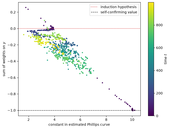
The beliefs spend most of their time near the self-confirming value (sum of weights \(\approx -1\)) but repeatedly shoot up toward the induction line (sum of weights \(= 0\)) — the escape route along which the government learns a Solow-Tobin version of the natural-rate hypothesis and stabilizes inflation.
89.7. Relation to equilibria under forecast misspecification#
The near-Ramsey episodes are reminiscent of the equilibria with optimal misspecified forecasts of Optimal Misspecified Beliefs and Self-Confirming Equilibria.
There, a forecasting model without a constant but with a unit root could closely approximate a true model that includes a constant.
Here an approximation with a similar flavor operates during the near-Ramsey episodes: the government’s estimated Phillips curve, by driving the sum of weights toward zero, uses the induction hypothesis to approximate a constant — except that the approximated model is not fixed but changes as the government’s own beliefs feed back through the Phelps problem.
89.8. Role of the discount factor#
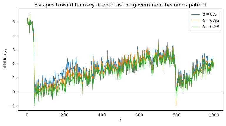
The recurrent stabilizations toward Ramsey depend on the discount factor \(\delta\) being near one.
Lowering \(\delta\) raises the inflation rate observed during the low-inflation episodes, consistent with the workings of the Phelps problem under the induction hypothesis.
fig, ax = plt.subplots(figsize=(9, 4.5))
for δ in [0.90, 0.95, 0.98]:
    m = AdaptivePhillips(δ=δ)
    sim = simulate(m, λ=0.975, T_prior=300, n=1000, seed=1)
    ax.plot(sim['y'], lw=0.7, label=rf'$\delta = {δ}$')
ax.axhline(0, color='k', lw=0.5)
ax.set_xlabel('$t$')
ax.set_ylabel('inflation $y_t$')
ax.legend()
ax.set_title('Escapes toward Ramsey deepen as the government becomes patient')
plt.show()
89.9. Anticipated utility#
The adaptive model is an example of what David Kreps calls an anticipated utility model [Kreps, 1998].
The government adapts a temporarily misspecified model — a Phillips curve with fixed coefficients — to incorporate the most recent observations, and reoptimizes along the way.
In forming decisions at \(t\), it acts as if its current estimate \(\gamma_{t-1}\) will govern the Phillips curve forever, using the same policy functional \(h(\cdot)\) that would be optimal if \(\gamma\) were truly time-invariant.
This is a small departure from rational expectations: calendar time enters only through the drifting beliefs \(\gamma_t\).
Unlike Bayesian or robust decision makers, an anticipated-utility government ignores its period-by-period model misspecification — it does not entertain the possibility that its coefficients will drift, even as they do.
Yet, as the simulations show, this modest departure from rationality is enough to generate a rich account of the rise and fall of U.S. inflation, and to supply underpinnings for the vindication of econometric policy evaluation.
89.10. Conclusions#
For long stretches, an adaptive government learns to generate better than Nash outcomes.
These results come from the recurrent dynamics of adaptation: the mean dynamics that under least squares pull the system toward a self-confirming equilibrium continue to operate, but under a constant gain the noise lets the system recurrently escape toward the Ramsey outcome.
Starting from a self-confirming equilibrium, the adaptive algorithm gradually makes the government put enough weight on the induction hypothesis that chance observations eventually promote a stabilization.
Adaptation makes the government’s beliefs a hidden state that imparts serial correlation into inflation and unemployment — so that an outside forecaster would do well to use a random-coefficients model, or to make the constant adjustments that Lucas noted in his Critique [Lucas, 1976].
In this sense the adaptive models contain the underpinnings for vindicating econometric policy evaluation — the second of the two stories of The Rise and Fall of U.S. Inflation.
89.11. Exercises#
Exercise 89.1
Build the Keynesian adaptive model, in which the government fits the Phillips curve in the reverse direction, regressing inflation on unemployment.
The regressors are \(X_{K,t} = \begin{bmatrix} U_t & U_{t-1} & U_{t-2} & y_{t-1} & y_{t-2} & 1 \end{bmatrix}'\), and the government estimates \(\beta\) in \(y_t = \beta' X_{K,t} + \varepsilon_{K,t}\), then inverts to \(\gamma\) before solving the Phelps problem.
Rather than re-derive everything, explore the classical model’s sensitivity to the constant gain: simulate with \(\lambda \in \{0.99, 0.975, 0.95\}\) and compare how often inflation escapes toward Ramsey.
How does a larger gain (smaller \(\lambda\), faster discounting of the past) affect the frequency of escapes?
Solution
fig, ax = plt.subplots(figsize=(9, 4.5))
for λ in [0.99, 0.975, 0.95]:
    sim = simulate(model, λ=λ, T_prior=300, n=1000, seed=1)
    frac = (sim['y'] < 2).mean()
    ax.plot(sim['y'], lw=0.6,
            label=rf'$\lambda = {λ}$ (near-Ramsey {frac:.0%})')
ax.axhline(0, color='k', lw=0.5)
ax.set_xlabel('$t$')
ax.set_ylabel('inflation $y_t$')
ax.legend()
plt.show()
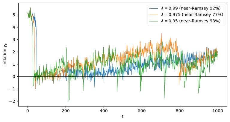
A larger constant gain (smaller \(\lambda\)) discounts the past more heavily, arresting convergence to the self-confirming equilibrium more forcefully and producing more frequent — though also noisier — escapes toward the Ramsey outcome.
Exercise 89.2
The contrast between Figures 8.1 and 8.2 hinges on the gain, but the least squares result also depends on the tightness of the prior.
Simulate the least squares system (\(\lambda = 1\)) for prior tightness \(T \in \{500, 2000, 5000\}\), and report the mean inflation rate across several seeds.
Explain why a looser prior (smaller \(T\)) makes even the least squares system prone to escapes.
Solution
for T in [500, 2000, 5000]:
    means = [simulate(model, λ=1.0, T_prior=T, n=1000, seed=s)['y'].mean()
             for s in range(6)]
    print(f"T = {T:>4}:  mean inflation across seeds = "
          f"{np.round(means, 1)}")
T =  500:  mean inflation across seeds = [0.9 1.9 5.  2.3 1.3 0.6]
T = 2000:  mean inflation across seeds = [4.7 5.  5.  5.  3.7 4.9]
T = 5000:  mean inflation across seeds = [5. 5. 5. 5. 5. 5.]
With a looser prior the effective gain \(1/(T + t)\) starts larger, so early updates are big enough to kick the beliefs off the self-confirming equilibrium.
Because that equilibrium is only marginally stable — the mean dynamics have an eigenvalue at the boundary of the region of fast convergence — the system can then drift toward the induction hypothesis and get stuck near Ramsey, mimicking the constant-gain escapes.
A tighter prior keeps the gain small throughout, so least squares reliably hugs the self-confirming equilibrium.