90. Escaping Nash Inflation#
90.1. Overview#
If an unlikely event occurs, it is very likely to occur in the most likely way.
– Michael Harrison
This lecture is the analytical completion of Adaptive Learning and Escape Dynamics.
It follows [Cho et al., 2002] (CWS), which turns the simulated escape dynamics of chapter 8 of [Sargent, 1999] into a deterministic characterization.
In Adaptive Learning and Escape Dynamics we watched a constant-gain government recurrently escape the Nash self-confirming equilibrium and spend long spells near the Ramsey outcome — but we described those escapes only informally and by simulation.
CWS show that the escapes are governed by their own ordinary differential equation, obtained from the theory of large deviations.
The picture that emerges has two deterministic pieces:
the mean dynamics, an ODE that pulls the government’s beliefs toward the self-confirming equilibrium; and
the escape dynamics, a second ODE that — driven by a “most likely unlikely” sequence of shocks — pushes beliefs away from it, toward the beliefs that support the Ramsey outcome.
The remarkable finding is that the escape has a dominant path: conditional on escaping, the government’s beliefs follow a nearly deterministic route along which it temporarily learns a version of the natural-rate hypothesis and cuts inflation.
This lecture is a technical extension of Adaptive Learning and Escape Dynamics; the next lecture, Priors, Escapes, and Learning Cycles, builds on it by asking how the government’s prior about parameter drift reshapes both the mean dynamics and these escape dynamics.
We work with the analytically tractable static model.
Let’s start with our imports:
import matplotlib.pyplot as plt
import numpy as np
from scipy.integrate import solve_ivp
90.2. The model#
The true economy is the natural-rate model of [Kydland and Prescott, 1977],
with \(\theta, u > 0\) and \(W_n = (W_{1n}, W_{2n})'\) i.i.d. standard Gaussian.
The government does not know (90.1).
In the static model it fits a non-expectational Phillips curve by regressing unemployment on inflation and a constant,
with beliefs \(\gamma = (\gamma_1, \gamma_{-1})\) (slope and intercept), and it treats \(\eta_n\) as exogenous.
Believing (90.2), the government solves the Phelps problem, whose static best response sets inflation to the constant
Three beliefs are worth naming, following CWS:
Belief 1 (Nash): \(\gamma_1 = -\theta\) with an intercept that makes \(x = \theta u\) — the time-consistent outcome of [Kydland and Prescott, 1977].
Belief 2 (Ramsey): \(\gamma_1 = 0\), so the government perceives no tradeoff and sets \(x = 0\).
Belief 3 (induction): coefficients on inflation summing to zero, which for a patient government also sends inflation to \(0\).
class EscapeModel:
    "CWS 2002 static model. γ = (γ₁ slope, γ₋₁ intercept), regressors Φ = (π, 1)."

    def __init__(self, θ=1.0, u=5.0, σ1=0.3, σ2=0.3):
        self.θ, self.u, self.σ1, self.σ2 = θ, u, σ1, σ2

    def x(self, γ):
        γ1, γm1 = γ
        return -γm1 * γ1 / (1 + γ1**2)

    def M(self, γ):
        "E[ΦΦ'] with Φ = (π, 1)."
        x = self.x(γ)
        return np.array([[x**2 + self.σ2**2, x], [x, 1.0]])

    def g_bar(self, γ):
        "Mean-dynamics forcing E[Φ(U − Φ'γ)] = M(T(γ) − γ)."
        x = self.x(γ)
        E_ΦU = np.array([x * self.u - self.θ * self.σ2**2, self.u])
        return E_ΦU - self.M(γ) @ γ
90.3. The self-confirming equilibrium#
A self-confirming equilibrium is a belief that reproduces itself: the population regression coefficients of (90.2), computed on the data the government generates by acting on \(\gamma\), equal \(\gamma\).
Writing \(T(\gamma)\) for those population coefficients, CWS show
so a self-confirming equilibrium solves \(\bar g(\gamma) = 0\).
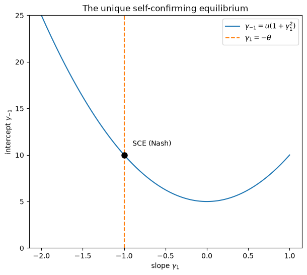
For the static model the equilibrium is the intersection of the line \(\gamma_1 = -\theta\) with the parabola \(\gamma_{-1} = u(1 + \gamma_1^2)\) — a unique point that supports the Nash outcome of The Credibility Problem.
It is the same self-confirming equilibrium constructed in Self-Confirming Equilibria, written here in the static (constant-plus-slope) special case that Priors, Escapes, and Learning Cycles also uses.
model = EscapeModel(θ=1.0, u=5.0, σ1=0.3, σ2=0.3)
γ_sce = np.array([-model.θ, model.u * (1 + model.θ**2)])

print(f"self-confirming beliefs γ = {γ_sce}  (slope -θ, intercept u(1+θ²))")
print(f"self-confirming inflation x = {model.x(γ_sce):.2f}  (= Nash = θu)")
print(f"check g_bar = {model.g_bar(γ_sce)}")
self-confirming beliefs γ = [-1. 10.]  (slope -θ, intercept u(1+θ²))
self-confirming inflation x = 5.00  (= Nash = θu)
check g_bar = [0. 0.]
γ1_grid = np.linspace(-2, 1, 200)
fig, ax = plt.subplots(figsize=(7, 6))
ax.plot(γ1_grid, model.u * (1 + γ1_grid**2), label=r'$\gamma_{-1} = u(1+\gamma_1^2)$')
ax.axvline(-model.θ, color='C1', ls='--', label=r'$\gamma_1 = -\theta$')
ax.plot(γ_sce[0], γ_sce[1], 'ko', ms=8)
ax.annotate('SCE (Nash)', γ_sce, (γ_sce[0] + 0.1, γ_sce[1] + 1))
ax.set_xlabel(r'slope $\gamma_1$')
ax.set_ylabel(r'intercept $\gamma_{-1}$')
ax.set_ylim(0, 25)
ax.legend()
ax.set_title('The unique self-confirming equilibrium')
plt.show()
90.4. Adaptation and the mean dynamics#
We make the government adaptive: each period it updates \(\gamma\) by constant-gain recursive least squares and acts on its current estimate — an anticipated-utility model in the sense of [Kreps, 1998].
The literature on least squares learning ([Marcet and Sargent, 1989], [Woodford, 1990], [Evans and Honkapohja, 2001]) shows that, as the gain \(\varepsilon \to 0\), the beliefs are approximated by the mean-dynamics ODE
A rest point of (90.4) is a self-confirming equilibrium, and CWS show this ODE is globally stable about it.
So under the mean dynamics alone, the adaptive government is drawn to Nash inflation.
def mean_ode(t, z, model):
    γ, R = z[:2], z[2:].reshape(2, 2)
    return np.concatenate([np.linalg.inv(R) @ model.g_bar(γ),
                           (model.M(γ) - R).ravel()])

z0 = np.concatenate([γ_sce + np.array([0.4, -3.0]), model.M(γ_sce).ravel()])
sol = solve_ivp(lambda t, z: mean_ode(t, z, model), [0, 60], z0,
                max_step=0.1, rtol=1e-9, atol=1e-11)

fig, ax = plt.subplots(figsize=(8, 4.5))
ax.plot(sol.t, -sol.y[1] * sol.y[0] / (1 + sol.y[0]**2))
ax.axhline(model.θ * model.u, color='k', ls='--', lw=1, label='Nash')
ax.set_xlabel('time')
ax.set_ylabel('inflation $x$')
ax.set_title('Mean dynamics: from a perturbed start, beliefs return to Nash')
ax.legend()
plt.show()
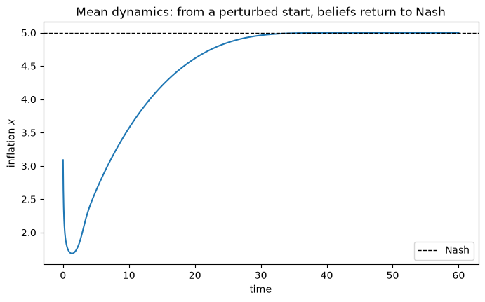
The mean dynamics cannot, on their own, explain the recurrent visits to low inflation in the simulations of Adaptive Learning and Escape Dynamics.
For that we need a second force.
90.5. Escape dynamics as a control problem#
Although the impact of the noise vanishes as \(\varepsilon \to 0\), for a fixed positive gain rare sequences of shocks can push beliefs a long way from the self-confirming equilibrium.
The theory of large deviations characterizes the most likely such rare event.
For a candidate belief path \(\gamma(\cdot)\), one defines a log-moment-generating (H-) functional of the least-squares innovations, its Legendre transform \(L\), and an action functional \(S(T, \gamma) = \int_0^T L\,ds\) that measures how “costly” — how improbable — the path is.
The dominant escape path minimizes the action subject to leaving a neighbourhood \(G\) of \(\bar\gamma\).
Drawing on [Williams, 2019], CWS reduce this to a clean control problem: the H-functional becomes a quadratic form with a normalizing matrix \(Q\) (a fourth-moment matrix obtained from Lyapunov equations), and the escape path solves
subject to the perturbed mean dynamics
Read (90.5) as a least squares problem: \(v\) is the extra “forcing” that the mean dynamics would need to escape, \(Q\) plays the role of a covariance matrix, and the least-cost forcing is the most likely unusual shock sequence.
Two consequences (their Theorem 5.3) tie the control problem to the stochastic model:
the probability of an escape on a bounded interval is \(\approx \exp(-\bar S/\varepsilon)\), so the mean time between escapes is \(\approx \exp(\bar S/\varepsilon)\); and
conditional on escaping, beliefs follow the dominant escape path with probability approaching one.
The escape dynamics, like the mean dynamics, are deterministic.
90.6. The dominant escape path#
For the static model with binomial shocks, CWS solve the control problem in closed form (their Section 7).
The escape forcing is strikingly simple:
so the dominant escape path solves
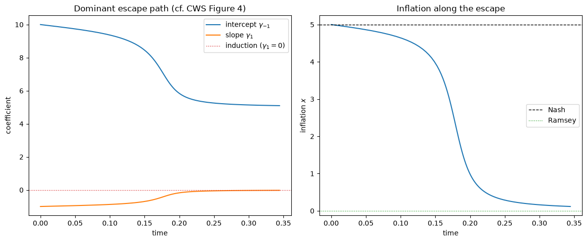
Let’s integrate (90.8) from the self-confirming equilibrium until beliefs leave a circle of radius 5.
def escape_ode(t, z, model):
    γ, R = z[:2], z[2:].reshape(2, 2)
    force = np.array([model.σ1 * model.σ2, 0.0])
    return np.concatenate([np.linalg.inv(R) @ (model.g_bar(γ) + force),
                           (model.M(γ) - R).ravel()])

def left_circle(t, z):
    "Terminal event: beliefs leave the radius-5 circle around the SCE."
    return 5.0 - np.linalg.norm(z[:2] - γ_sce)
left_circle.terminal = True
left_circle.direction = -1

z0 = np.concatenate([γ_sce, model.M(γ_sce).ravel()])
esc = solve_ivp(lambda t, z: escape_ode(t, z, model), [0, 200], z0,
                events=left_circle, max_step=0.02, rtol=1e-9, atol=1e-11)

slope, intercept = esc.y[0], esc.y[1]
infl = -intercept * slope / (1 + slope**2)
fig, axes = plt.subplots(1, 2, figsize=(12, 5))

axes[0].plot(esc.t, intercept, label='intercept $\\gamma_{-1}$')
axes[0].plot(esc.t, slope, label='slope $\\gamma_1$')
axes[0].axhline(0, color='C3', ls=':', lw=1, label='induction ($\\gamma_1 = 0$)')
axes[0].set_xlabel('time')
axes[0].set_ylabel('coefficient')
axes[0].set_title('Dominant escape path (cf. CWS Figure 4)')
axes[0].legend()

axes[1].plot(esc.t, infl)
axes[1].axhline(model.θ * model.u, color='k', ls='--', lw=1, label='Nash')
axes[1].axhline(0, color='C2', ls=':', lw=1, label='Ramsey')
axes[1].set_xlabel('time')
axes[1].set_ylabel('inflation $x$')
axes[1].set_title('Inflation along the escape')
axes[1].legend()

plt.tight_layout()
plt.show()
print(f"slope     : {slope[0]:.2f} → {slope[-1]:.3f}   (induction hypothesis at 0)")
print(f"intercept : {intercept[0]:.1f} → {intercept[-1]:.1f}")
print(f"inflation : {infl[0]:.2f} → {infl[-1]:.2f}   (Nash {model.θ*model.u:.0f} → Ramsey 0)")
slope     : -1.00 → -0.023   (induction hypothesis at 0)
intercept : 10.0 → 5.1
inflation : 5.00 → 0.12   (Nash 5 → Ramsey 0)
Along the dominant escape path the slope rises from its self-confirming value of \(-1\) toward zero — the induction hypothesis — and inflation falls from the Nash value toward Ramsey.
This is exactly the temporary stabilization we saw by simulation in Adaptive Learning and Escape Dynamics, now derived as a deterministic path: the government, by chance, generates enough inflation experiments to discover a good-enough version of the natural-rate hypothesis, and acts on it.
90.7. The race of four ODEs#
Where does the escape forcing (90.7) come from?
With binomial shocks \(W_{in} \in \{-1, +1\}\), the shock pair realized in any period lies in one of four groups.
CWS show that the most likely escape uses the same unusual pair repeatedly, so there are four candidate escape ODEs — one per pair — and the dominant escape is the one that reaches the boundary fastest.
Let’s compute the instantaneous velocity of each candidate at the self-confirming equilibrium.
R0 = model.M(γ_sce)
R0_inv = np.linalg.inv(R0)
σ1σ2 = model.σ1 * model.σ2

candidates = {
    "{(1,1),(-1,-1)}  → Ramsey": np.array([σ1σ2, 0.0]),
    "{(1,-1),(-1,1)}  → higher π": np.array([-σ1σ2, 0.0]),
    "{(1,1),(1,-1)}": R0 @ (R0_inv @ np.array([model.x(γ_sce) * model.σ1, model.σ1])),
    "{(-1,1),(-1,-1)}": R0 @ (R0_inv @ np.array([-model.x(γ_sce) * model.σ1, -model.σ1])),
}

for name, force in candidates.items():
    v = R0_inv @ force
    print(f"  {name:28s}  |velocity| = {np.linalg.norm(v):.3f}")
  {(1,1),(-1,-1)}  → Ramsey     |velocity| = 5.099
  {(1,-1),(-1,1)}  → higher π   |velocity| = 5.099
  {(1,1),(1,-1)}                |velocity| = 0.300
  {(-1,1),(-1,-1)}              |velocity| = 0.300
The pair \(\{(1,1), (-1,-1)\}\) produces a velocity far larger than the last two, and it points toward Ramsey (rising slope, falling intercept).
Its mirror image \(\{(1,-1),(-1,1)\}\) has the same speed but points the wrong way — toward higher inflation — where the mean dynamics oppose it and quickly pull it back.
So the winner of the race is the Ramsey-ward path, and the escape forcing it induces is the \(R^{-1}(\sigma_1\sigma_2, 0)'\) of (90.7).
90.8. Mean dynamics reinforce the escape#
Why does the Ramsey-ward escape succeed while its mirror image fails?
Near the self-confirming equilibrium the mean dynamics point toward it, opposing any escape.
But CWS (their Figures 8-9) show that once beliefs have moved a little way out along the Ramsey-ward direction, the mean dynamics themselves start pointing toward Ramsey, reinforcing the escape.
We can see this by plotting the mean-dynamics vector field in belief space.
gs = np.linspace(-1.2, 0.1, 16)      # slope
gi = np.linspace(4.5, 10.5, 16)      # intercept
GS, GI = np.meshgrid(gs, gi)
DS, DI = np.zeros_like(GS), np.zeros_like(GI)

for i in range(GS.shape[0]):
    for j in range(GS.shape[1]):
        γ = np.array([GS[i, j], GI[i, j]])
        d = np.linalg.inv(model.M(γ)) @ model.g_bar(γ)
        DS[i, j], DI[i, j] = d

fig, ax = plt.subplots(figsize=(8, 6))
ax.quiver(GS, GI, DS, DI, angles='xy', alpha=0.7)
ax.plot(*γ_sce, 'ko', ms=8, label='SCE (Nash)')
ax.plot(0, model.u, 'C2s', ms=8, label='Ramsey belief')
ax.plot(slope, intercept, 'C3', lw=2, label='escape path')
ax.set_xlabel(r'slope $\gamma_1$')
ax.set_ylabel(r'intercept $\gamma_{-1}$')
ax.set_title('Mean dynamics (arrows) and the escape path')
ax.legend()
plt.show()
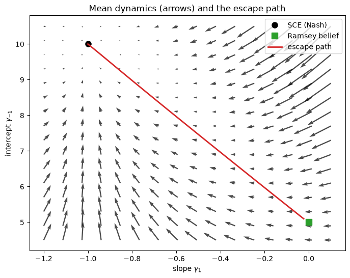
Near the self-confirming equilibrium the arrows push back toward Nash, but away from it — along the escape route — they sweep toward the Ramsey belief.
The escape dynamics only need to start the departure; the mean dynamics finish the job.
This is the sense in which the mean dynamics trace a circuitous route: pushed off the equilibrium along the escape path, the system travels near Ramsey before the residual short-run Phillips curve is rediscovered and the mean dynamics eventually carry beliefs back to Nash.
90.9. The experimentation trap#
The escape has a compelling behavioural interpretation.
Within its approximating model, the government can only detect the natural-rate hypothesis if there is enough dispersion in inflation.
But inside a self-confirming equilibrium the government sets a constant systematic inflation rate, so it generates no such dispersion — it is caught in an experimentation trap.
Only an unusual run of shocks makes the government vary inflation enough to steepen its estimated Phillips curve; a steeper perceived curve leads it (through the best response) to cut inflation, which generates further influential observations that steepen the curve further.
This self-reinforcing process halts when the perceived Phillips curve is vertical — the induction hypothesis — and inflation is near Ramsey.
The system cannot stay there forever: in truth there is a short-run Phillips curve, which the government eventually rediscovers, rekindling the mean dynamics that carry it back to Nash.
90.10. Escape frequency and model richness#
The minimized action \(\bar S\) governs how often escapes occur: the mean escape time grows like \(\exp(\bar S/\varepsilon)\).
A striking finding of CWS is that escapes are more frequent when the government’s model is richer.
The full dynamic model of Adaptive Learning and Escape Dynamics — with lagged unemployment and inflation — has a much smaller \(\bar S\) than the static model, even though the two share the same self-confirming equilibrium.
A richer model lets the government detect the subtler distributed-lag (“induction-hypothesis”) version of the natural-rate hypothesis, so it escapes toward Ramsey more readily.
Note
The escape dynamics inherit the same “near determinism” that makes the mean dynamics useful: for small gains, the stochastic simulations of Adaptive Learning and Escape Dynamics hug the deterministic escape path derived here. The next lecture, Priors, Escapes, and Learning Cycles, shows that the government’s prior about how its coefficients drift reshapes both dynamics — and can even make the escape a deterministic cycle.
90.11. Escaping volatile inflation#
The escape delivers a fall in the level of inflation.
[Ellison and Yates, 2007] extend the model to explain a second post-war fact: inflation volatility rose and fell together with the level.
Their device is to give the government a reason to stabilize.
Following [Phelps and Taylor, 1977], they add an unemployment shock \(W_3\) that the government — but not the price-setting private sector — can react to.
Now a government that believes in an exploitable Phillips curve is tempted to lean against \(W_3\) by varying inflation, so the perceived effectiveness of policy, \(|\gamma_1|\), drives the volatility of inflation as well as its level.
In their model the expected inflation volatility a private agent faces is
At the self-confirming equilibrium \(\gamma_1 = -\theta\), the government believes policy is effective and leans against \(W_3\) aggressively, so inflation is volatile.
Along an escape, \(\gamma_1 \to 0\): the government stops believing it can exploit the Phillips curve, abandons stabilization, and the volatility term collapses to the control error \(\sigma_2\).
Applying (90.9) to the belief path we already computed shows the level and volatility of inflation escaping in tandem.
σ3 = 0.9                                   # size of the stabilizable shock
infl_vol = np.sqrt(model.σ2**2 + (slope / (1 + slope**2))**2 * σ3**2)

fig, axes = plt.subplots(1, 2, figsize=(12, 4.5))
axes[0].plot(esc.t, infl)
axes[0].axhline(model.θ * model.u, color='k', ls='--', lw=1, label='Nash')
axes[0].axhline(0, color='C2', ls=':', lw=1, label='Ramsey')
axes[0].set_xlabel('time'); axes[0].set_ylabel('inflation level')
axes[0].set_title('level escapes'); axes[0].legend()

axes[1].plot(esc.t, infl_vol, 'C1')
axes[1].axhline(model.σ2, color='k', ls='--', lw=1, label=r'control error $\sigma_2$')
axes[1].set_xlabel('time'); axes[1].set_ylabel('inflation volatility')
axes[1].set_title('volatility escapes too'); axes[1].legend()

plt.tight_layout()
plt.show()
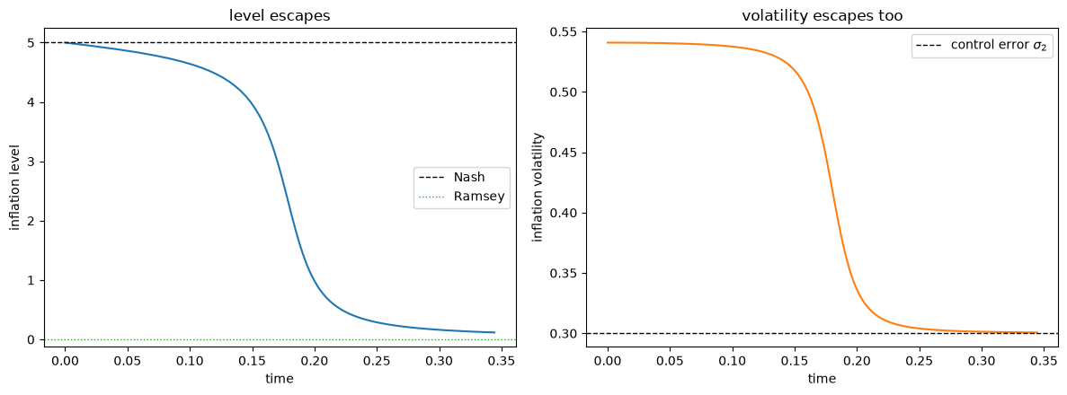
Both fall as beliefs escape, because both spring from the same source: the government’s belief in an exploitable tradeoff.
[Ellison and Yates, 2007] draw a further, subtler lesson about the timing of escapes.
A larger stabilizable shock \(\sigma_3\) makes an escape harder to trigger: to create the illusion that inflation moves while unemployment stays put, an unusual sequence of shocks must now offset not only the control errors but also the government’s own stabilizing reaction to \(W_3\).
The more shocks the government can offset, the more complex the escape-triggering sequence, and the longer the wait.
Taken literally, this says an economy is more likely to escape to low inflation precisely when there are few shocks to stabilize — a suggestive link between the arrival of the mid-1980s calm and the disinflation that accompanied it.
90.12. Exercises#
Exercise 90.1
The escape forcing (90.7) scales with \(\sigma_1 \sigma_2\) — the product of the two shock standard deviations.
Integrate the dominant escape ODE (90.8) for a grid of \(\sigma_1 = \sigma_2 = \sigma \in \{0.2, 0.3, 0.4, 0.5\}\) and report, for each, the exit time from the radius-5 circle.
How does a noisier economy affect how quickly beliefs travel along the escape route?
Solution
for σ in [0.2, 0.3, 0.4, 0.5]:
    m = EscapeModel(θ=1.0, u=5.0, σ1=σ, σ2=σ)
    γ0 = np.array([-m.θ, m.u * (1 + m.θ**2)])

    def leave(t, z, m=m, γ0=γ0):
        return 5.0 - np.linalg.norm(z[:2] - γ0)
    leave.terminal = True
    leave.direction = -1

    z0 = np.concatenate([γ0, m.M(γ0).ravel()])
    s = solve_ivp(lambda t, z: escape_ode(t, z, m), [0, 500], z0,
                  events=leave, max_step=0.02, rtol=1e-9, atol=1e-11)
    print(f"σ = {σ}: exit time along the escape path = {s.t[-1]:.2f}")
σ = 0.2: exit time along the escape path = 0.20
σ = 0.3: exit time along the escape path = 0.34
σ = 0.4: exit time along the escape path = 0.50
σ = 0.5: exit time along the escape path = 0.67
A larger \(\sigma\) makes the escape forcing \(R^{-1}(\sigma_1\sigma_2, 0)'\) stronger, so beliefs travel the escape route faster (a shorter exit time along the deterministic path).
Note that this is distinct from the frequency of escapes, which is governed by the action \(\bar S\) and the gain \(\varepsilon\); a noisier economy travels a given escape route more quickly once the escape is under way.
Exercise 90.2
Make the reinforcement in the vector-field plot quantitative.
At several points along the escape path, evaluate the mean-dynamics drift \(R^{-1}\bar g(\gamma)\) and measure its cosine alignment with the direction from the current beliefs toward the Ramsey belief \((0, u)\).
A cosine near \(+1\) means the mean dynamics are pushing beliefs toward Ramsey — reinforcing the escape.
Solution
γ_ramsey = np.array([0.0, model.u])            # Belief 2

def cosine_toward_ramsey(γ, R):
    drift = np.linalg.inv(R) @ model.g_bar(γ)
    to_ramsey = γ_ramsey - γ
    denom = np.linalg.norm(drift) * np.linalg.norm(to_ramsey)
    return np.nan if denom < 1e-9 else drift @ to_ramsey / denom

for frac in [0.0, 0.25, 0.5, 0.75, 0.95]:
    k = min(int(frac * len(esc.t)), len(esc.t) - 1)
    γ, R = esc.y[:2, k], esc.y[2:, k].reshape(2, 2)
    print(f"frac {frac:.2f}:  γ = ({γ[0]:+.2f}, {γ[1]:.1f}),  "
          f"cos(drift, →Ramsey) = {cosine_toward_ramsey(γ, R):+.2f}")
frac 0.00:  γ = (-1.00, 10.0),  cos(drift, →Ramsey) = +nan
frac 0.25:  γ = (-0.65, 8.2),  cos(drift, →Ramsey) = +1.00
frac 0.50:  γ = (-0.23, 6.1),  cos(drift, →Ramsey) = +1.00
frac 0.75:  γ = (-0.07, 5.3),  cos(drift, →Ramsey) = +1.00
frac 0.95:  γ = (-0.03, 5.1),  cos(drift, →Ramsey) = +1.00
Right at the self-confirming equilibrium the drift vanishes (the cosine is undefined), so the mean dynamics neither help nor hinder.
But once beliefs have moved even slightly along the escape route, the mean-dynamics drift points almost exactly toward the Ramsey belief (cosine \(\approx +1\)): the mean dynamics reinforce the escape all the way to Ramsey.
The opposition that CWS emphasize is confined to a tiny neighbourhood of the equilibrium — the escape dynamics only need to nudge beliefs out of it, after which the mean dynamics finish the job.