84. The Rise and Fall of U.S. Inflation #

In addition to what’s in Anaconda, this lecture will use the following libraries to download and filter macroeconomic data:

!pip install pandas_datareader

84.1. Overview #

This is the first lecture in a suite based on Thomas Sargent’s The Conquest of American Inflation [Sargent, 1999].

It combines chapters 1 and 2 of that book.

The suite asks a question about post-war U.S. macroeconomic history:

If we take for granted that inflation is under the control of the Federal Reserve, how can we explain the rise of U.S. inflation into the 1970s and its abrupt fall under Paul Volcker in the early 1980s?

The essay evaluates two interpretations, both based on policy makers’ beliefs about the Phillips curve.

In both stories, the Federal Reserve learns the natural-rate-of-unemployment theory from a combination of experience and a priori reasoning.

The stories differ in how that theory is cast:

The triumph of natural-rate theory. Academic economists discovered the natural-rate hypothesis, taught that any inflation-unemployment tradeoff is temporary, and eventually persuaded policy makers to pursue low inflation.
The vindication of econometric policy evaluation. Policy makers never abandoned the methods that Robert Lucas criticized in his famous Critique. Recurrently re-estimating a Phillips curve and using it to choose a target, they were led by the data itself — an adversely shifting empirical Phillips curve — toward lower inflation.

This lecture presents the facts that motivate both stories, sketches the two interpretations, and reviews the Lucas Critique that chapter 2 both invokes and modifies.

The remaining lectures in the suite build the models:

The Credibility Problem — the one-period Kydland-Prescott credibility problem (chapter 3).
Adaptive Expectations and the Phelps Problem — adaptive expectations and the Phelps problem (chapter 5).
Optimal Misspecified Beliefs — equilibrium under optimal misspecified beliefs (chapter 6).
Self-Confirming Equilibria — self-confirming equilibria (chapter 7).
Adaptive Learning and Escape Dynamics — adaptive learning, escape dynamics, and simulated Volcker stabilizations (chapter 8).
Escaping Nash Inflation — the escape dynamics characterized analytically ([Cho et al., 2002]).
Priors, Escapes, and Learning Cycles — how the government’s prior about drifting coefficients shapes convergence, cycles, and escapes ([Sargent and Williams, 2005]).
The Lost Conquest: Fed Policy in the 2020s — the same tools turned on the 2020s inflation and the Fed’s slow response ([Sargent and Williams, 2025]).
Drifts and Volatilities — an empirical postscript that fits a drifting-coefficient, stochastic-volatility VAR to the data and asks whether the Great Inflation was bad policy or bad luck ([Cogley and Sargent, 2005]).

Let’s start with some imports:

import matplotlib.pyplot as plt
import numpy as np
import pandas as pd
import datetime
from pandas_datareader import data as web
from statsmodels.tsa.filters.bk_filter import bkfilter

Note

The figures in the next two sections reproduce the ones in chapters 1 and 2 of [Sargent, 1999], which were drawn from data available in the late 1990s. We download the underlying series from FRED and restrict attention to the same historical window. The section Data patterns after 1999 then carries the most enlightening of these figures through to the present and asks what the additional quarter-century of data means for the two stories.

84.2. Facts #

We begin with the single fact that the whole essay seeks to explain: the hump-shaped path of U.S. inflation since World War II.

We measure inflation by the annualized monthly change in the consumer price index (all items), smoothed with a 13-month centered moving average to remove seasonal and high-frequency noise.

start, end = datetime.datetime(1948, 1, 1), datetime.datetime(1999, 1, 1)

cpi = web.DataReader('CPIAUCNS', 'fred', start, end)['CPIAUCNS']

# annualized monthly inflation, then a 13-month centered moving average
inflation = 1200 * np.log(cpi).diff()
inflation_ma = inflation.rolling(13, center=True).mean()

fig, ax = plt.subplots(figsize=(9, 5))
ax.plot(inflation_ma, lw=1.2)
ax.axhline(0, color='k', lw=0.5)
ax.set_xlabel('year')
ax.set_ylabel('inflation (percent, annualized)')
ax.set_title('Figure 1.1: Monthly inflation, CPI all items, '
             '13-month centered moving average')
plt.show()

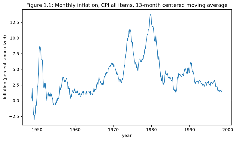
_images/c9816a33e5afedc694f370b722daa133c8e952c8034d9bcd11a9851fab1fa1ef.png

Inflation was low during the late 1950s and early 1960s, swept upward into the 1970s, and then fell abruptly with Volcker’s stabilization in the early 1980s.

Any explanation that treats inflation as under the Federal Reserve’s control must account for this rise and fall.

84.3. The Phillips curve in the data #

Despite its disrepute in some academic and policy-making circles, the Phillips curve persists in U.S. data, and simple procedures detect it.

To coax the Phillips curve from the data, we follow the book in two ways.

First, we use the unemployment rate for a single demographic group — white men 20 years and over — rather than the aggregate rate, which is contaminated by slow-moving shifts in the demographic mix.

Second, we look at business-cycle frequencies, filtering out slowly moving components so that the eye can spot the inverse relationship between inflation and unemployment.

u = web.DataReader('LNS14000028', 'fred', start, end)['LNS14000028']  # white men 20+

data = pd.concat([inflation.rename('inflation'),
                  u.rename('unemployment')], axis=1).dropna()
data.head()

	inflation	unemployment
DATE
1954-01-01	0.000000	3.6
1954-02-01	0.000000	3.8
1954-03-01	0.000000	4.1
1954-04-01	-4.469279	4.7
1954-05-01	4.469279	4.6

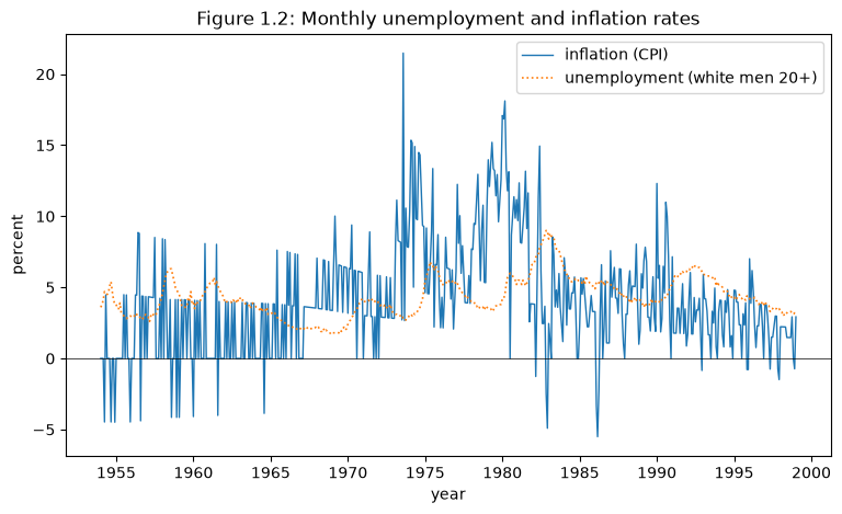
Figure 1.2 plots the two raw series together.

fig, ax = plt.subplots(figsize=(9, 5))
ax.plot(data.index, data['inflation'], 'C0', lw=1, label='inflation (CPI)')
ax.plot(data.index, data['unemployment'], 'C1:', lw=1.2,
        label='unemployment (white men 20+)')
ax.axhline(0, color='k', lw=0.5)
ax.set_xlabel('year')
ax.set_ylabel('percent')
ax.set_title('Figure 1.2: Monthly unemployment and inflation rates')
ax.legend()
plt.show()

_images/a98ef6ce069a5f54e15850488bd13fc113c498254ac36193c99d7588d35a49ab.png

To isolate the business-cycle relationship, we apply the finite-lag bandpass filter of Baxter and King [Baxter and King, 1999].

Following the book, we keep fluctuations with periods between 24 and 84 months and use a lead-lag truncation of 84 months.

# Baxter-King bandpass: periods between 24 and 84 months, truncation 84
bk = bkfilter(data, low=24, high=84, K=84)
bk.columns = ['inflation_cycle', 'unemployment_cycle']

fig, ax = plt.subplots(figsize=(9, 5))
ax.plot(bk.index, bk['inflation_cycle'], 'C0', lw=1, label='inflation')
ax.plot(bk.index, bk['unemployment_cycle'], 'C1:', lw=1.2,
        label='unemployment')
ax.axhline(0, color='k', lw=0.5)
ax.set_xlabel('year')
ax.set_ylabel('deviation from trend (percent)')
ax.set_title('Figure 1.3: Business-cycle components '
             '(Baxter-King bandpass filter)')
ax.legend()
plt.show()

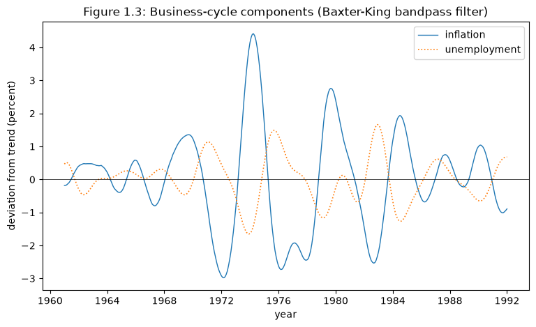
_images/e245ce54f8fc8a67758e779cd430801d85138c5d6bf20c5fa7dc2869bb124f9a.png

The filtered components tend to move in opposite directions: a business-cycle Phillips curve.

We can see the tradeoff more directly in a scatter plot for the subperiod that interests us most, 1960-1982.

Figure 1.4 plots the raw series against each other, and Figure 1.5 the business-cycle components.

sub = slice('1960', '1982')

fig, axes = plt.subplots(1, 2, figsize=(12, 5))

axes[0].scatter(data.loc[sub, 'inflation'],
                data.loc[sub, 'unemployment'], s=8, alpha=0.6)
axes[0].set_xlabel('inflation')
axes[0].set_ylabel('unemployment (white men 20+)')
axes[0].set_title('Figure 1.4: Raw series, 1960-1982')

axes[1].scatter(bk.loc[sub, 'inflation_cycle'],
                bk.loc[sub, 'unemployment_cycle'], s=8, alpha=0.6)
axes[1].set_xlabel('inflation (business-cycle component)')
axes[1].set_ylabel('unemployment (business-cycle component)')
axes[1].set_title('Figure 1.5: Business-cycle components, 1960-1982')

plt.tight_layout()
plt.show()

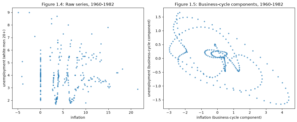
_images/3d840b4fa0cfdcba4c7352d6e0a4f3379f7679db7278e2c70c9821ecb0a60e8a.png

Focusing on the business-cycle components sharpens the apparent Phillips curve.

Figure 1.5 reveals Phillips loops: inflation and unemployment trace out counter-clockwise loops rather than a single stable curve, a signature of the shifting expectations that the natural-rate theory places at the center of the story.

Note

The book adjusts for demographic change by choosing a single unemployment series. A broader definition of unemployment would inject additional low-frequency demographic components, which one might model with a unit-root process. The essay instead puts a unit root into the inflation-unemployment process from a different source: the drifting beliefs of a monetary authority cut loose from the discipline of Bretton Woods.

84.4. Two interpretations #

Both stories start from the same initial conditions — the history of inflation and unemployment, and the state of expectations, inherited by policy makers around 1960 — and both assume that the data conform to the natural-rate hypothesis, whether or not policy makers realized it.

84.4.1. The triumph of natural-rate theory#

Adherence to the gold standard and then to Bretton Woods gave the U.S. low inflation and low expected inflation.

In 1960, Paul Samuelson and Robert Solow [Samuelson and Solow, 1960] found a Phillips curve in U.S. data and taught that it was exploitable — that policy could raise inflation to reduce unemployment.

Within a decade this recommendation was widely endorsed and implemented.

To everyone’s dismay, the Phillips curve then shifted adversely: inflation rose, but unemployment on average did not fall.

Meanwhile Edmund Phelps [Phelps, 1967], Milton Friedman [Friedman, 1968], and Robert Lucas [Lucas, 1972] created and refined the concept of the natural rate of unemployment, which assigns a central role to expectations of inflation in locating the Phillips curve.

The natural-rate theory allowed only a temporary tradeoff and explained the adverse shifts; its rational expectations version implied that policy makers should ignore the temporary tradeoff and strive only for low inflation.

In this story, these ideas diffused from academics to policy makers and ultimately produced the lower inflation of the 1980s and 1990s.

Events were shaped by policy makers’ beliefs — some false, others true — and the actions those beliefs inspired.

84.4.2. The vindication of econometric policy evaluation#

The alternative story ascribes Volcker’s conquest partly to the success of the very econometric and policy-making procedures that Lucas challenged.

Policy makers accepted the Samuelson-Solow Phillips curve as an exploitable tradeoff and adopted their methods for learning from data and deducing policy.

Recurrently, they re-estimated a distributed-lag Phillips curve and used it to reset a target inflation-unemployment pair.

Interpreted mechanically — without identifying expectations as the hidden state variable — the adversely shifting empirical Phillips curve eventually led policy makers to pursue lower inflation.

This story is told with an adaptive theory of policy that departs minimally from rational expectations.

It connects a sequence of ideas that the rest of the suite develops: drifting coefficients, self-confirming equilibria, least squares and other recursive learning algorithms, convergence of least squares learners to self-confirming equilibria, and recurrent dynamics along escape routes from those equilibria.

The key idea, taken from Christopher Sims [Sims, 1988], is that an adaptive model lets a government learn from its past attempts to exploit the Phillips curve, and eventually discover a version of the natural-rate hypothesis that instructs it to reduce inflation.

84.5. Ignoring the Lucas Critique #

Chapter 2 of the book confronts the obvious objection to the vindication story: doesn’t the Lucas Critique forbid the mechanical, exploitable Phillips curve on which it rests?

The essay resurrects the econometric and policy-evaluation procedures that Lucas decisively criticized [Lucas, 1976], and emphasizes a neglected aspect of his Critique: drifting coefficients.

84.5.1. The Critique#

An econometric model is a collection of stochastic difference equations, some of which describe private agents’ decision rules.

Econometric policy evaluation in the Tinbergen-Theil tradition holds those private decision rules fixed while the government optimizes its own rule against an objective function.

Lucas noted that if private agents solve intertemporal optimization problems, their decision rules depend on the government’s rule.

By missing this dependence, the Tinbergen-Theil method mistranslates the government’s preferences over outcomes into an ordering over decision rules, and so gives unreliable policy advice.

84.5.2. The appeal to drifting coefficients#

Lucas conceded the impressive forecasting record of Keynesian models but argued that good forecasting is no evidence for the invariance under intervention that Tinbergen-Theil assumes.

He stressed that forecasters routinely adjusted the constant terms of key equations, and interpreted these adjustments as an adaptive-coefficients model in the spirit of Cooley and Prescott [Cooley and Prescott, 1973].

The intertemporal instability of estimated relationships — coefficient drift — undermined treating them as invariant to systematic changes in policy rules.

Yet Lucas left the drift unexplained, and neither the macroeconomic theory nor the rational expectations econometrics built after the Critique accounts for it: both focus on environments with time-invariant transition functions.

84.5.3. Parameter drift as a point of departure#

The essay starts from parameter drift, treating it as a smoking gun — the key evidence that the government’s beliefs about the economy, and hence its policy toward inflation, have evolved over time.

It builds a model from two components:

a Tinbergen-Theil theory of government decision making — the Phelps problem of Adaptive Expectations and the Phelps Problem; and
a drifting-coefficients econometric procedure for the government, featuring the constant adjustments that Lucas wrote about.

Within a self-confirming equilibrium (developed in Self-Confirming Equilibria), some of the force of the Lucas Critique vanishes.

Although the government’s invariance assumption is wrong, it is not disappointed in outcomes, because those outcomes are statistically consistent with its beliefs.

A self-confirming equilibrium is a rational expectations equilibrium with fewer free parameters than the models Lucas used — and precisely those lost parameters would be needed to represent regime changes.

To admit regime changes and drifting coefficients, convergence to a self-confirming equilibrium must be resisted.

The essay arrests convergence by replacing the government’s least squares estimator with a constant-gain, adaptive-coefficients algorithm that overweights recent data — endowing the government with a suspicion that the environment is unstable.

This weakens the pull toward a self-confirming equilibrium and sustains dynamics along an escape route, along which regime changes occur.

Ironically, as we shall see in Adaptive Learning and Escape Dynamics, the procedures that violate the Lucas Critique can yield better outcomes than ones that respect it.

84.6. A premature summary: triumph or vindication?#

The rest of this suite builds models.

Before we start, it is worth previewing where they lead and the tension they leave unresolved — a premature summary of the journey, adapted from the concluding chapter of [Sargent, 1999].

Everything can be organized around two benchmark models.

In the first, due to [Phelps, 1967], the public forms expectations adaptively while the government chooses policy optimally, taking the public’s rule as given.

In the second, the rational-expectations natural-rate model, the public is rational while the government’s policy is treated as exogenous and arbitrary.

Lucas recommended replacing the first benchmark with the second.

Coming to grips with the two stories drives us to propose models that make various compromises between these poles — and the remaining lectures are those compromises.

84.6.1. The road ahead#

We begin, in The Credibility Problem, by imposing rationality on both sides.

The one-period [Kydland and Prescott, 1977] model delivers a pessimistic prediction — the high-inflation time-consistent (Nash) outcome — but a repeated-economy version of the theory of credible policy replaces that pessimism with agnosticism: so many outcomes become sustainable that the theory yields only weak predictions.

That weakness is the first reason to hesitate before declaring the triumph of natural-rate theory.

We then turn back from the Lucas Critique and start again from the Phelps benchmark, but with one change: the government’s model of the private sector is no longer arbitrary — it is fit to historical data.

Varying the details of that fitting problem generates the rest of the suite:

self-confirming equilibria (Self-Confirming Equilibria),
equilibria with optimally misspecified forecasting functions (Optimal Misspecified Beliefs), and
adaptive, “anticipated-utility” learning models (Adaptive Learning and Escape Dynamics, Escaping Nash Inflation, and Priors, Escapes, and Learning Cycles).

These adaptive models are a disciplined retreat from rational expectations, not an abandonment of it.

They carry no free parameters governing expectations; period by period they impose the same cross-equation restrictions as a rational expectations model; and — because a self-confirming equilibrium is the attractor of their mean dynamics — they converge back to rational expectations under tranquil conditions, satisfying a desideratum of [Kreps, 1998].

But, following [Sims, 1988], our real interest is in the recurrent dynamics that adaptation adds.

Suspecting that the Phillips curve is prone to wander, the government uses a constant-gain algorithm, which is the sensible choice when coefficients drift.

The payoff is a striking one: the adaptive models produce abrupt stabilizations of inflation that defy the inferior self-confirming outcome toward which the mean dynamics point.

These regime shifts arise not from any change in the government’s procedures, nor from large shocks, but from changes in beliefs created by the government’s own econometrics — the mathematics of escape routes in the space of approximating models.

84.6.2. The induction hypothesis: villain and hero#

At the center of the story sits the induction hypothesis — the restriction that the weights on lagged inflation in an expectations equation sum to one, so that a permanently higher inflation rate is eventually fully expected.

It was built almost without comment into the adaptive expectations hypothesis of [Friedman, 1957] and [Cagan, 1956], and it was the basis of Solow’s and Tobin’s early tests of the natural-rate hypothesis [Solow, 1968, Tobin, 1968].

Cast as a villain in Lucas’s Critique — a naive restriction that rational expectations does not imply — the induction hypothesis re-emerges as the hero of the adaptive models: activating it is exactly what makes the government’s Phelps problem call for near-Ramsey, low-inflation policy.

The escape routes our simulations follow are precisely the paths along which the government’s estimated model, by using a unit root to approximate a constant, stumbles into believing the induction hypothesis.

Wrestling with such approximation problems, with several models simultaneously in play, is what led [Sims, 1980] to call bounded rationality a wilderness, set apart from the tidy one-model world of rational expectations.

84.6.3. The reservation#

Which story, then — triumph or vindication?

The contest is not rational expectations versus an alternative, because both stories selectively apply and withdraw from rational expectations.

And the vindication story, however well it fits, is an exercise in positive economics, not normative economics.

It is tempting to read its long stretches of near-Ramsey inflation as an endorsement of the adaptive policy-making procedures that produce them — but that temptation should be resisted.

For the same mean dynamics that permit a stabilization also guarantee that it is temporary: once beliefs drift close enough to the induction hypothesis, the mean dynamics begin to point away from it, back toward the region where the Phelps problem recommends resuscitating inflation.

The simulations contain long episodes that look like Paul Volcker — and others that look like Arthur Burns.

Theoretical work after [Kydland and Prescott, 1977], and [Rogoff, 1985], insists that durable low inflation must rest on commitment mechanisms that keep a monetary authority from choosing sequentially — not on the hope that an adaptive government, armed with an approximate model, will by chance eventually learn to do approximately the right thing.

So the book ends on a hope rather than a verdict: we hope that the triumph story is the right one — that policy makers have learned a correct rational expectations version of the natural-rate hypothesis and have found devices to commit themselves to low inflation.

Because if instead the vindication story is closer to the truth, then the same mean dynamics that carried inflation down are always waiting, eventually, to carry it back up.

The quarter-century of data since 1999 — a long, quiet Great Moderation interrupted by a sudden surge in 2021-2022 — is a running test of exactly this hope, and we turn to it next.

84.7. Data patterns after 1999 #

[Sargent, 1999] was written at the end of the long disinflation that began with Volcker.

We now have another quarter-century of data.

This section carries the book’s most enlightening figures through to the present and asks what the new observations mean for the two stories.

Let’s extend the sample to the latest available month.

end_recent = datetime.datetime(2026, 7, 1)

cpi_full = web.DataReader('CPIAUCNS', 'fred', start, end_recent)['CPIAUCNS']
u_full = web.DataReader('LNS14000028', 'fred', start, end_recent)['LNS14000028']

# the book's measure (annualized monthly change, 13-month centered MA)
inflation_full = 1200 * np.log(cpi_full).diff()
inflation_ma_full = inflation_full.rolling(13, center=True).mean()

# year-over-year inflation: smoother, and the measure usually quoted today
inflation_yoy = 100 * (cpi_full / cpi_full.shift(12) - 1)

84.7.1. The rise and fall, extended#

Figure 1.1 showed inflation rising into the 1970s and falling under Volcker.

Extending it to the present adds three chapters the book could not see: the Great Moderation of low, stable inflation from the mid-1980s; a long spell near — and briefly below — zero after the 2008 financial crisis; and a sudden surge in 2021-2022 to the highest rate since 1981, followed by a rapid decline.

fig, ax = plt.subplots(figsize=(11, 5))
ax.plot(inflation_ma_full, lw=1)
ax.axhline(0, color='k', lw=0.5)
ax.axvspan(pd.Timestamp('1948-01-01'), pd.Timestamp('1999-01-01'),
           color='C0', alpha=0.06, label="the book's window")
for date, y, txt in [('1980-03-01', 13.7, '1970s\nacceleration'),
                     ('1983-06-01', 3.0, 'Volcker'),
                     ('2009-07-01', -1.5, '2009\ndeflation scare'),
                     ('2022-06-01', 8.9, '2021-22\nsurge')]:
    ax.annotate(txt, (pd.Timestamp(date), y), ha='center', fontsize=9,
                color='C3')
ax.set_xlabel('year')
ax.set_ylabel('inflation (percent, annualized)')
ax.set_title('Inflation, CPI all items, 13-month centered moving average, '
             '1948-2026')
ax.legend(loc='upper right')
plt.show()

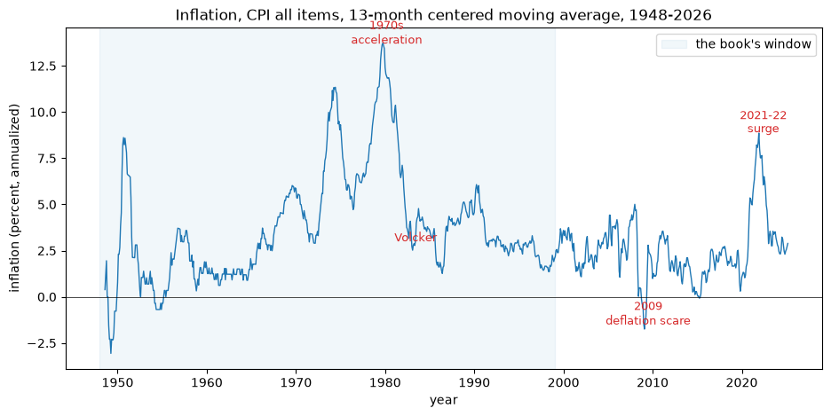
_images/82ecdb3c470040dccb205357c268573e9e1446a9162109fdf110c5c3be676901.png

The hump that the book set out to explain is now one of two.

The second, in 2021-2022, is a genuinely new episode — a fast acceleration and an almost-as-fast disinflation, all compressed into about three years.

84.7.2. Unemployment and inflation to the present#

Figure 1.2 plotted the two series together for the post-war period.

Extending it shows the two most dramatic macroeconomic events of the new data: the COVID unemployment spike of 2020 — briefly the highest since the Great Depression — and the inflation surge that followed.

recent = slice('1990', None)

fig, ax = plt.subplots(figsize=(11, 5))
ax.plot(inflation_yoy[recent], 'C0', lw=1, label='inflation (CPI, year-over-year)')
ax.plot(u_full[recent], 'C1:', lw=1.2, label='unemployment (white men 20+)')
ax.axhline(0, color='k', lw=0.5)
ax.set_xlabel('year')
ax.set_ylabel('percent')
ax.set_title('Unemployment and inflation, 1990-2026')
ax.legend()
plt.show()

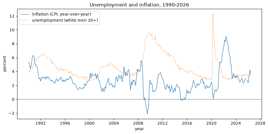
_images/36aef23028f5c6e2418058ca8e4cc86c715d14854cdc9672e63c27a5fc404267.png

Two features stand out.

From the mid-1990s to 2020, inflation stayed remarkably quiet even as unemployment swung widely — falling to historic lows in the late 1990s and 2019, and doubling in the 2008 recession.

Then, after the COVID spike, unemployment fell back quickly and inflation surged — a pattern with the fingerprints of a supply disturbance rather than the demand-driven tradeoff of the classic Phillips curve.

84.7.3. The Phillips curve across three eras#

The book coaxed a Phillips curve from 1960-1982 data.

The most striking post-1999 pattern is how unstable the inflation-unemployment scatter has been across eras.

We split the sample into the book’s acceleration era, the Great Moderation, and the post-2008 period, and plot inflation against unemployment in each.

scatter_data = pd.concat([inflation_yoy.rename('inflation'),
                          u_full.rename('unemployment')], axis=1).dropna()

eras = [('1960', '1983', '1960-1983 (acceleration)'),
        ('1984', '2007', '1984-2007 (Great Moderation)'),
        ('2008', None, '2008-2026 (crisis, COVID, surge)')]

fig, axes = plt.subplots(1, 3, figsize=(14, 4.5), sharex=True, sharey=True)
for ax, (lo, hi, title) in zip(axes, eras):
    era_data = scatter_data.loc[lo:hi]
    ax.scatter(era_data['unemployment'], era_data['inflation'], s=8, alpha=0.5)
    ax.axhline(0, color='k', lw=0.5)
    ax.set_xlabel('unemployment')
    ax.set_title(title, fontsize=10)
axes[0].set_ylabel('inflation (year-over-year)')
plt.tight_layout()
plt.show()

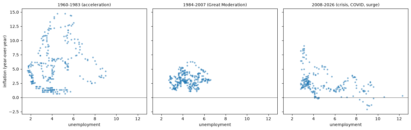
_images/2f000569fd33adab3c9814643f0df50d5f46b1e6648f40fa771bacb975e3e462.png

The three clouds could hardly look more different.

In 1960-1983 the points sprawl across a wide range of inflation rates — the era of shifting expectations and Phillips loops.

In 1984-2007 they collapse into a tight, low, nearly flat cloud — the Great Moderation, in which inflation barely responded to unemployment at all.

Since 2008 the relationship dissolves into a scatter dominated by two outliers: the COVID recession, with double-digit unemployment and still-low inflation, and the 2021-2022 surge, with high inflation and low unemployment.

Whatever the Phillips curve is, it is not a stable structural relationship — exactly the instability that motivates the book’s account of drifting beliefs.

84.7.4. What the new data mean for the two stories#

The additional quarter-century neither refutes nor confirms either story cleanly, but it sharpens both.

For the triumph of natural-rate theory. The Great Moderation reads as the triumph completed: with the natural-rate consensus entrenched and central-bank independence established, inflation stayed low and expectations stayed anchored for a generation.

In the book’s language, the economy settled into a low-inflation self-confirming equilibrium and stayed there.

Even the 2021-2022 surge, on this reading, supports the triumph: once the Federal Reserve moved decisively, inflation came down quickly and long-run expectations never came unmoored — the low-inflation equilibrium survived a large shock.

For the vindication of econometric policy evaluation. The surge is also a reminder that the monetary authority’s model can still mislead it: the widely-held 2021 view that inflation would be “transitory” was a model that the data falsified, and policy adjusted only after beliefs did.

The decade of near-zero inflation before 2020 — the apparently flat Phillips curve, with neither the “missing disinflation” of 2009-2013 nor the “missing inflation” of 2015-2019 fitting a stable curve — is precisely the kind of drifting empirical relationship whose changing slope and intercept the book’s adaptive government tracks in real time.

Note

A caveat the book itself would insist on: its mechanisms assume that the fundamentals — the true data-generating process — are stable, so that all the action comes from the government’s evolving beliefs. The 2021-2022 episode involved genuine supply shocks (pandemic disruptions, energy prices), which lie outside that assumption. Disentangling shifting beliefs from shifting fundamentals is exactly the identification problem that makes this history so hard, and so interesting.

The tools built in the rest of this suite — self-confirming equilibria, drifting coefficients, and escape dynamics — remain a natural language for asking the question the new data pose: will a credible low-inflation equilibrium keep re-anchoring after each shock, or can a sequence of surprises still set beliefs drifting, as they did after 1965?

The final lecture, The Lost Conquest: Fed Policy in the 2020s, turns exactly these tools on the 2021-2022 surge, and asks why the Federal Reserve was so slow to respond.

84.8. Exercises #

Exercise 84.1

The claim that “focusing on the business-cycle components sharpens the apparent Phillips curve” can be made quantitative.

Compute the correlation between inflation and unemployment over 1960-1982 for

the raw series (as in Figure 1.4), and
the Baxter-King business-cycle components (as in Figure 1.5).

By how much does bandpass filtering sharpen the negative Phillips correlation?

Solution

corr_raw = data.loc[sub].corr().iloc[0, 1]
corr_cycle = bk.loc[sub].corr().iloc[0, 1]

print(f"raw correlation, 1960-1982        : {corr_raw:+.2f}")
print(f"business-cycle correlation, 1960-82: {corr_cycle:+.2f}")

raw correlation, 1960-1982        : +0.03
business-cycle correlation, 1960-82: -0.64

In the raw series the correlation is close to zero: the adverse shifts of the Phillips curve — the slowly moving expectational component that the natural-rate theory emphasizes — swamp the business-cycle tradeoff.

Once those low-frequency shifts are filtered out, a strong negative relationship emerges, confirming that the Phillips tradeoff operates at business-cycle frequencies.