86. Adaptive Expectations and the Phelps Problem#
In addition to what’s in Anaconda, this lecture will use the following library:
!pip install quantecon
86.1. Overview#
They cannot look out far. They cannot look in deep. But when was that ever a bar To any watch they keep?
– Robert Frost
This lecture continues the study of Phillips curve tradeoffs begun in The Credibility Problem.
It follows chapter 5 of [Sargent, 1999].
We describe
the Cagan-Friedman adaptive expectations hypothesis,
how [Phelps, 1967] used it to formulate a government control problem, and
the role of adaptive expectations in early econometric tests of the natural-rate hypothesis.
The key object is the Phelps problem: a government that is rational solves an optimal control problem while the public forecasts inflation with a fixed, mechanical adaptive rule.
Unlike the one-period model of The Credibility Problem, the government now takes into account that the economy lasts more than one period, and that today’s inflation shapes tomorrow’s expectations.
This intertemporal link can improve outcomes and, in a limiting case, even sustain the Ramsey outcome.
The Phelps problem is a linear-quadratic (LQ) control problem, so we solve it with the LQ control tools from QuantEcon.
Let’s start with some imports:
import matplotlib.pyplot as plt
import numpy as np
import quantecon as qe
86.2. Adaptive expectations#
[Phelps, 1967] formulated a control problem for a natural-rate model.
He dropped rationality for the public but not for the government, and assigned the public a particular mechanical forecasting rule that is known to the government.
The public uses the adaptive expectations scheme of Milton Friedman and [Cagan, 1956]:
where \(x_t\) is the public’s expectation of inflation and \(y_t\) is inflation.
Rearranging, \(x_t = \lambda x_{t-1} + (1 - \lambda) y_{t-1}\), so expected inflation is a geometric distributed lag of past inflation,
Notice that (86.1) is a constant gain version of the least squares learning algorithm from The Credibility Problem, with the constant \((1 - \lambda)\) playing the role that the decreasing gain \(t^{-1}\) played there.
Equation (86.2) possesses an induction property: if the government keeps repeating a constant \(y_t = \tilde y\) policy, eventually the public comes to set \(x_t \approx \tilde y\).
The weights \((1 - \lambda)\lambda^{i-1}\) sum to one, so a permanently maintained inflation rate is eventually expected.
Let’s confirm the induction property numerically.
def adaptive_forecast(y, λ, x0=0.0):
    "Simulate x_t = λ x_{t-1} + (1-λ) y_{t-1}."
    T = len(y)
    x = np.empty(T)
    x[0] = x0
    for t in range(1, T):
        x[t] = λ * x[t - 1] + (1 - λ) * y[t - 1]
    return x

T = 60
y_const = np.full(T, 10.0)                 # a constant inflation policy

fig, ax = plt.subplots(figsize=(9, 4.5))
for λ in [0.7, 0.9]:
    x = adaptive_forecast(y_const, λ)
    ax.plot(x, lw=1.5, label=rf'$\lambda = {λ}$')
ax.axhline(10.0, color='k', ls='--', lw=1, label='policy $\\tilde y$')
ax.set_xlabel('$t$')
ax.set_ylabel('expected inflation $x_t$')
ax.legend()
plt.show()
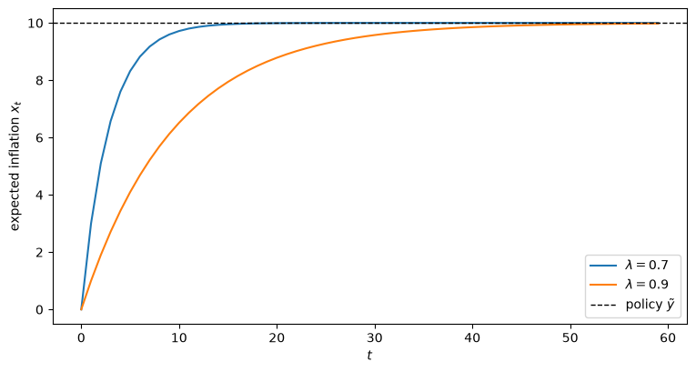
Under a constant policy the public’s expectation converges to the policy, more slowly the larger is \(\lambda\).
Solow and Tobin exploited this induction property when they tested the natural-rate hypothesis, as we discuss below.
86.3. The Phelps problem#
The economy repeats forever, and the government evaluates outcome sequences with the discounted criterion
When \(\delta = 1\) we interpret (86.3) in the limit-of-means (Cesàro) sense.
The government maximizes (86.3) by choice of a rule for inflation \(y_t\), subject to the adaptive expectations scheme (86.1) and the expectations-augmented Phillips curve
Because expected inflation \(x_t\) is predetermined at the start of period \(t\), it is the only endogenous state variable.
The government’s problem is therefore a discounted LQ control problem with
state \(s_t = \begin{bmatrix} 1 & x_t \end{bmatrix}'\),
control \(y_t\), and
transition \(x_{t+1} = \lambda x_t + (1 - \lambda) y_t\).
86.3.1. Casting the problem in LQ form#
Write \(U_t = a' s_t - \theta y_t\) with \(a = \begin{bmatrix} U^* & \theta \end{bmatrix}'\).
The per-period loss \(\tfrac{1}{2}(U_t^2 + y_t^2)\) then equals
Matching this to the QuantEcon LQ loss \(s_t' R s_t + y_t' Q y_t + 2 y_t' N s_t\), and matching the transition to \(s_{t+1} = A s_t + B y_t\), gives
The discount factor is \(\beta = \delta\); the scaling \((1 - \delta)\) in (86.3) does not affect the optimal policy.
class PhelpsProblem:
    """
    The Phelps optimal-control problem: a rational government facing a
    public that forecasts inflation adaptively with parameter λ.
    """

    def __init__(self, θ=1.0, U_star=5.0, λ=0.7, δ=0.96):
        self.θ, self.U_star, self.λ, self.δ = θ, U_star, λ, δ

        a = np.array([[U_star], [θ]])
        R = 0.5 * (a @ a.T)
        Q = np.array([[0.5 * (θ**2 + 1)]])
        N = -0.5 * θ * a.T
        A = np.array([[1.0, 0.0], [0.0, λ]])
        B = np.array([[0.0], [1 - λ]])

        # δ = 1 (limit of means) is handled as the limit δ → 1
        β = min(δ, 1 - 1e-7)
        self.lq = qe.LQ(Q, R, A, B, N=N, beta=β)
        P, F, d = self.lq.stationary_values()

        # optimal rule y_t = f1 + f2 x_t
        self.f1, self.f2 = -F[0, 0], -F[0, 1]

    def simulate(self, x0=12.0, T=60):
        "Disinflation path (U_t, y_t) starting from expectation x0."
        θ, U_star, λ = self.θ, self.U_star, self.λ
        U, y, x = np.empty(T), np.empty(T), x0
        for t in range(T):
            y[t] = self.f1 + self.f2 * x
            U[t] = U_star - θ * (y[t] - x)
            x = λ * x + (1 - λ) * y[t]
        return U, y
The optimal rule takes the form \(y_t = f_1 + f_2 x_t\) with \(f_1 \neq 0\) and \(f_2 \neq 1\).
These inequalities reflect that the public does not use an optimal forecasting rule; if instead \(f_1 = 0\) and \(f_2 = 1\), we would have \(y_t = x_t\) for all histories.
pp = PhelpsProblem(θ=1.0, U_star=5.0, λ=0.7, δ=0.96)
print(f"optimal rule:  y_t = {pp.f1:.3f} + {pp.f2:.3f} x_t")
optimal rule: y_t = 0.406 + 0.334 x_t
86.3.2. A proposition#
The reason the Phelps problem is interesting is the following result.
Proposition 86.1 (δ = 1 eventually sustains Ramsey)
In the absence of discounting (\(\delta = 1\)), the government drives \(y_t\) to \(0\), the Ramsey outcome.
When \(\delta = 1\), \(\lambda\) governs the speed of convergence to the Ramsey outcome.
When \(\delta < 1\), the limit point of \(y_t\) depends on a comparison of \(\lambda\) with \(\delta\).
For \(\lambda < \delta\) and \(\delta\) close to \(1\), the government’s policy eventually approximates the Ramsey outcome.
The public’s expectations are wrong along the transition path but are correct in the steady state, by virtue of the induction property.
86.4. Disinflation paths#
We now reproduce the disinflation experiments of chapter 5 of [Sargent, 1999].
Set \(\theta = 1\) and \(U^* = 5\), and start the government’s problem from late-1970s initial conditions \(x_{-1} = y_{-1} = 12\), which imply \(U = U^* = 5\).
The following tables record paths of unemployment \(U\) and inflation \(y\) at selected lags, for two discount factors \(\delta \in \{0.96, 1\}\) and two adaptation parameters \(\lambda \in \{0.7, 0.9\}\).
def disinflation_table(δ, lags=(1, 5, 20, 50)):
    rows = []
    for λ in [0.7, 0.9]:
        U, y = PhelpsProblem(λ=λ, δ=δ).simulate(x0=12.0, T=max(lags) + 1)
        for lag in lags:
            rows.append((λ, lag, U[lag - 1], y[lag - 1]))
    return rows

for δ in [0.96, 1.0]:
    print(f"\n δ = {δ}")
    print(f" {'λ':>4} {'lag':>4} {'U':>7} {'y':>7}")
    for λ, lag, U, y in disinflation_table(δ):
        print(f" {λ:>4} {lag:>4} {U:>7.1f} {y:>7.1f}")
 δ = 0.96
    λ  lag       U       y
  0.7    1    12.6     4.4
  0.7    5     8.1     2.2
  0.7   20     5.1     0.7
  0.7   50     5.0     0.6
  0.9    1    11.9     5.1
  0.9    5    10.2     4.3
  0.9   20     6.9     2.5
  0.9   50     5.3     1.6

 δ = 1.0
    λ  lag       U       y
  0.7    1    13.2     3.8
  0.7    5     8.3     1.5
  0.7   20     5.1     0.0
  0.7   50     5.0     0.0
  0.9    1    13.4     3.6
  0.9    5    11.3     2.7
  0.9   20     7.1     0.9
  0.9   50     5.2     0.1
For each parameter setting the government engineers a major recession and immediately brings inflation down more than halfway toward its eventual limiting value.
In the discounted case (\(\delta = 0.96\)), inflation settles at a positive level, and the government accepts a longer but milder recession when \(\lambda = 0.9\) than when \(\lambda = 0.7\).
In the undiscounted case (\(\delta = 1\)), inflation is driven all the way to the Ramsey value of zero, more slowly the larger is \(\lambda\).
Let’s plot the full disinflation paths.
fig, axes = plt.subplots(1, 2, figsize=(11, 4.5))

for δ, ax in zip([0.96, 1.0], axes):
    for λ in [0.7, 0.9]:
        U, y = PhelpsProblem(λ=λ, δ=δ).simulate(x0=12.0, T=60)
        ax.plot(y, lw=1.5, label=rf'$\lambda = {λ}$')
    ax.set_title(rf'$\delta = {δ}$')
    ax.set_xlabel('$t$')
    ax.set_ylabel('inflation $y_t$')
    ax.legend()

plt.tight_layout()
plt.show()
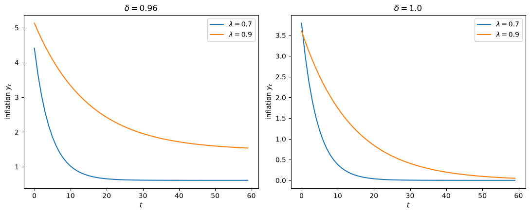
The undiscounted problem drives inflation to the Ramsey outcome; the discounted problem stops short of it.
86.5. The general Phelps problem#
For the government’s control problem, what matters is the reduced form of the Phillips curve, not the underlying structure that identifies \(x_t\).
It is useful to state a more general version of the Phelps problem in which the government’s model is a reduced-form distributed lag Phillips curve.
Define the vectors
and the state vector \(X_t = \begin{bmatrix} X_{U,t}' & X_{y,t}' & 1 \end{bmatrix}'\), which collects information dated \(t-1\) and earlier.
We can write two reduced-form Phillips curves that differ only in their direction of fit:
The subscripts \(C\) and \(K\) stand for Classical (regress \(U\) on \(y\)) and Keynesian (regress \(y\) on \(U\)).
The general Phelps problem is to choose a control law \(\hat y_t = h X_{t-1}\) to maximize the expected value of (86.3) subject to the government’s believed Phillips curve and to \(y_t = \hat y_t + v_{2t}\), where \(v_{2t}\) is a control error.
This induces a mapping from the government’s beliefs \(\gamma\) to its decision rule \(h\):
The specific problem solved above is the special case in which \(\gamma\) is restricted by substituting the adaptive expectations hypothesis (86.1) into the Phillips curve (86.4).
Once that substitution is made, the state variable \(x_t\) disappears from view.
These objects — \(\gamma\), \(\beta\), \(h(\gamma)\), and the two directions of fit — are exactly the ingredients we will need to define self-confirming equilibria in Self-Confirming Equilibria.
Note
The induction hypothesis is the restriction that, in the Keynesian Phillips curve \(y_t = \beta' X_{K,t} + \varepsilon_{K,t}\), the weights on lagged \(y\)’s sum to unity (equivalently, in the classical form the weights on current and lagged \(y\)’s sum to zero). Under adaptive expectations this holds because the weights in (86.2) sum to one.
86.6. Testing the natural-rate hypothesis#
Robert Solow and James Tobin [Solow, 1968, Tobin, 1968] exploited the induction hypothesis to test the natural-rate hypothesis.
Substituting the geometric distributed lag (86.2) into an inverted Phillips curve gives
They proposed to test the natural-rate hypothesis by running the regression
and interpreting a finding of \(b_1 < 1\) as evidence of a long-run tradeoff between inflation and unemployment of slope \(b_1 - 1\).
Early implementations found \(b_1 < 1\) and so rejected the natural-rate hypothesis in favor of a long-run tradeoff.
[King and Watson, 1994] and others later argued that the pattern of rejections and non-rejections is consistent with the tendency of inflation to have a unit root after the 1960s but not before, so the unit-sum restriction \(b_1 = 1\) is compatible with rational expectations when \(y_t\) has a unit root.
From the viewpoint of Phelps’s control problem, it is incidental whether the natural-rate hypothesis holds: the Phelps problem imparts interesting dynamics to the inflation-unemployment choice whether or not \(b_1 = 1\).
86.7. Sacrifice ratios and the subversion of the Phelps model#
Despite its encouraging implications for sustaining the Ramsey outcome under the induction hypothesis, Phelps’s control problem carries a tattered past.
In the Phelps problem, for a fixed \(\delta < 1\) it is always possible to find a \(\lambda\) close enough to 1 that high inflationary expectations will make a government want to avoid disinflating.
In the late 1970s, models with long expectations-adjustment lags were used to recommend against reducing inflation.
Large sacrifice ratios — estimated amounts of foregone GDP required to bring inflation down one percentage point — circulated widely.
The lesson to carry forward is that activating the induction hypothesis can eventually lead to better outcomes, but in the form that Phelps, Tobin, and Solow used it, the induction hypothesis retreats from rational expectations.
In Optimal Misspecified Beliefs and Self-Confirming Equilibria we impute more symmetry to the government and the public, applying updating schemes like (86.1) to functions rather than to numbers, and we turn \(\lambda\) from a free parameter into an equilibrium outcome.
The LQ Phelps problem solved here returns again in Adaptive Learning and Escape Dynamics, Escaping Nash Inflation, and Priors, Escapes, and Learning Cycles, where a learning government re-solves it every period — and where activating the induction hypothesis is exactly what triggers the Volcker-like stabilizations.
86.8. Exercises#
Exercise 86.1
The proposition above states that as \(\delta \to 1\) the government drives inflation to the Ramsey value \(0\).
For \(\lambda = 0.8\), compute the limiting inflation rate \(y_\infty\) (the value that \(y_t\) settles at after a long simulation) for a grid of discount factors \(\delta \in \{0.90, 0.92, \ldots, 0.99\}\).
Plot \(y_\infty\) against \(\delta\) and confirm that it declines toward zero as \(\delta \to 1\).
Solution
δ_grid = np.arange(0.90, 0.995, 0.01)
y_inf = []
for δ in δ_grid:
    U, y = PhelpsProblem(λ=0.8, δ=δ).simulate(x0=12.0, T=400)
    y_inf.append(y[-1])

fig, ax = plt.subplots(figsize=(8, 4.5))
ax.plot(δ_grid, y_inf, 'o-')
ax.set_xlabel(r'discount factor $\delta$')
ax.set_ylabel(r'limiting inflation $y_\infty$')
plt.show()
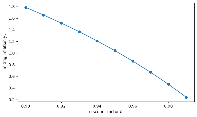
As \(\delta\) rises toward one, the government becomes willing to accept the transitional recession needed to reap the long-run benefit of low expected inflation, so the limiting inflation rate falls toward the Ramsey value of zero.
Exercise 86.2
Verify the induction property of the optimal policy directly.
Take the discounted problem with \(\delta = 0.96\) and \(\lambda = 0.7\), and simulate a long disinflation path.
Check that in the steady state the public’s expectation \(x_t\) equals actual inflation \(y_t\) (so the public is not fooled in the limit), even though expectations are wrong along the transition.
Solution
pp = PhelpsProblem(θ=1.0, U_star=5.0, λ=0.7, δ=0.96)
U, y = pp.simulate(x0=12.0, T=200)

# reconstruct the expectation path implied by the adaptive rule
x = adaptive_forecast(np.concatenate([[12.0], y]), λ=0.7, x0=12.0)[1:]

print(f"steady-state inflation   y_∞ = {y[-1]:.4f}")
print(f"steady-state expectation x_∞ = {x[-1]:.4f}")
print(f"gap                          = {y[-1] - x[-1]:.2e}")
steady-state inflation   y_∞ = 0.6098
steady-state expectation x_∞ = 0.6098
gap                          = -2.22e-16
In the steady state expected and actual inflation coincide, confirming that the induction property makes the public’s forecast correct in the limit.