85. The Credibility Problem#
85.1. Overview#
This lecture describes a basic expectational Phillips curve model of the sort studied by [Kydland and Prescott, 1977] and Robert Barro and David Gordon.
It is the first in a suite of lectures based on chapters of [Sargent, 1999].
Those chapters formalize
the temptation to inflate that is unleashed by the discovery of a Phillips curve,
the value of a commitment technology for resisting that temptation, and
the fragility of reputational mechanisms as substitutes for commitment.
Throughout, rational expectations is the only equilibrium concept that we use.
Alterations in the timing of decisions by a government and a private sector induce different economies with distinct outcomes.
A government faces a credibility problem whenever it wishes to make decisions sooner than it must.
We shall compare outcomes under two timing protocols:
In one, the government chooses inflation before the private sector sets its expectations, so the government takes into account how its choice shapes those expectations.
In the other, the government chooses inflation after the private sector has set its expectations.
The deterioration in outcomes under the second protocol measures the loss from an inability to commit.
We also study two out-of-equilibrium dynamics that converge to the no-commitment (Nash) outcome:
best response dynamics, and
least squares learning.
Let’s start with some standard imports:
import matplotlib.pyplot as plt
import numpy as np
85.2. A one-period economy#
Although credibility problems are intrinsically dynamic, it is possible to describe them in a one-period model under different patterns of within-period timing.
This prepares the way for the multi-period analyses in subsequent lectures.
We describe a version of the one-period model of [Kydland and Prescott, 1977] in the terms used by Nancy Stokey [Stokey, 1989].
Let \((U, y, x)\) be the unemployment rate, the inflation rate, and the public’s expectation of the inflation rate, respectively.
The government’s one-period payoff is
Unemployment is determined by an expectations-augmented Phillips curve
The equation asserts that unemployment deviates from \(U^*\), the natural rate, only when there is surprise inflation or deflation.
Substituting (85.2) into (85.1) expresses the government’s payoff as a function \(r(x, y)\):
We work with the following objects.
Rational expectations equilibrium: a triple \((U, x, y)\) satisfying (85.2) and \(y = x\).
Government (one-period) best response: given the public’s expectation \(x\), a decision rule \(B(x) = \operatorname{argmax}_y r(x, y)\) for setting \(y\).
Nash equilibrium: a pair \((x, y)\) satisfying (i) \(x = y\), and (ii) \(y = B(x)\).
Ramsey problem: \(\max_y r(y, y)\). The Ramsey outcome is the value of \(y\) that attains the maximum.
Best response dynamics: the dynamical system \(y_t = B(y_{t-1})\), \(y_0\) given.
A rational expectations equilibrium is a \((U, x, y)\) triple that lies on the Phillips curve and for which private agents are not fooled, given \(x\).
Substituting \(x = y\) into the Phillips curve (85.2) shows that \(U = U^*\) in any rational expectations equilibrium.
This identifies \(U^*\) as the natural rate of unemployment.
85.3. Nash and Ramsey outcomes#
A Nash equilibrium builds in a best response by the government, taking the state of expectations \(x\) as given, together with a response \(x = y\) by the market, i.e., rational expectations for a given \(y\).
Maximizing (85.3) with respect to \(y\) for a fixed \(x\) gives the government’s best response function
The Nash equilibrium sets \(x = y = B(x)\), which gives
The Ramsey problem instead imposes \(x = y\) before maximizing, so it maximizes \(r(y, y) = -\tfrac{1}{2}(U^{*2} + y^2)\), which yields the Ramsey outcome
Thus \(r(x^R, y^R) = -\tfrac{1}{2} U^{*2}\) while \(r(x^N, y^N) = -\tfrac{1}{2}(1 + \theta^2) U^{*2}\).
Both outcomes deliver the natural rate \(U^*\), but the Nash equilibrium delivers it with positive inflation and hence a strictly lower payoff.
Let’s collect these formulas in a class.
class CredibilityModel:
    """
    A one-period expectational Phillips curve economy.
    """

    def __init__(self, θ=1.0, U_star=5.0):
        self.θ, self.U_star = θ, U_star

    def phillips(self, y, x):
        "Unemployment implied by inflation y and expected inflation x."
        return self.U_star - self.θ * (y - x)

    def r(self, x, y):
        "Government one-period payoff."
        U = self.phillips(y, x)
        return -0.5 * (U**2 + y**2)

    def B(self, x):
        "Government best response to expected inflation x."
        θ = self.θ
        return θ / (θ**2 + 1) * self.U_star + θ**2 / (θ**2 + 1) * x

    def nash(self):
        "Nash equilibrium inflation (= expected inflation)."
        return self.θ * self.U_star

    def ramsey(self):
        "Ramsey inflation (= expected inflation)."
        return 0.0
cm = CredibilityModel()

y_N, y_R = cm.nash(), cm.ramsey()
print(f"Nash inflation      y^N = {y_N:.2f}")
print(f"Ramsey inflation    y^R = {y_R:.2f}")
print(f"Nash payoff         r   = {cm.r(y_N, y_N):.3f}")
print(f"Ramsey payoff       r   = {cm.r(y_R, y_R):.3f}")
Nash inflation      y^N = 5.00
Ramsey inflation    y^R = 0.00
Nash payoff         r   = -25.000
Ramsey payoff       r   = -12.500
The Nash payoff is worse than the Ramsey payoff.
The government would prefer the Ramsey outcome, but it cannot attain it without a technology for committing to \(y = 0\) before the public forms its expectations.
The Nash equilibrium is supported by a timing protocol in which the government decides after the private sector sets its expectations.
The Ramsey outcome is associated with a timing protocol in which the government chooses first, knowing that in a rational expectations equilibrium the public’s expectations will move with its choice because \(y = x\).
85.3.1. A picture of the two outcomes#
The government’s indifference curves are circles centered at the origin in \((U, y)\) space, because the payoff (85.1) depends only on \(U^2 + y^2\).
For a given expectation \(x\), the Phillips curve (85.2) is a downward-sloping line in \((U, y)\) space.
The government’s best response for \(y\), given \(x\), occurs where an indifference curve is tangent to the Phillips curve indexed by \(x\).
fig, ax = plt.subplots(figsize=(7, 6))

U_grid = np.linspace(0, 12, 200)

# a family of Phillips curves indexed by expected inflation x
for x in [0.0, y_N / 2, y_N]:
    # U = U_star - θ (y - x)  =>  y = x + (U_star - U) / θ
    y_line = x + (cm.U_star - U_grid) / cm.θ
    ax.plot(U_grid, y_line, 'C0', lw=1)

# government indifference curves (circles U^2 + y^2 = const)
ξ = np.linspace(0, 2 * np.pi, 200)
for R in [y_R, np.hypot(cm.U_star, y_N)]:
    if R > 0:
        ax.plot(R * np.cos(ξ), R * np.sin(ξ), 'C1--', lw=1)

ax.plot(cm.U_star, y_N, 'ko')
ax.annotate('Nash', (cm.U_star, y_N), (cm.U_star + 0.4, y_N + 0.4))
ax.plot(cm.U_star, y_R, 'ko')
ax.annotate('Ramsey', (cm.U_star, y_R), (cm.U_star + 0.4, y_R + 0.4))

ax.set_xlim(0, 12)
ax.set_ylim(0, 10)
ax.set_xlabel('unemployment $U$')
ax.set_ylabel('inflation $y$')
plt.show()
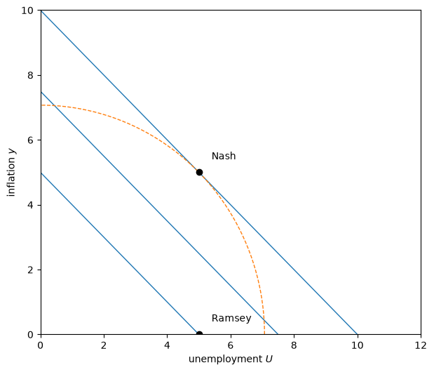
Solid lines are Phillips curves for expected inflation \(x \in \{0, y^N/2, y^N\}\); dashed circles are government indifference curves.
The Nash outcome \((U^*, y^N)\) lies on a larger circle (lower payoff) than the Ramsey outcome \((U^*, 0)\).
85.4. Best response dynamics#
Best response dynamics convert the one-period model into a dynamic one by positing an adaptive mechanism in which expected inflation equals last period’s inflation, \(x_t = y_{t-1}\).
This leads to the dynamics
Because \(B\) is an affine map with slope \(\theta^2 / (\theta^2 + 1) \in (0, 1)\), iterating on it converges to the fixed point \(y^N = \theta U^*\) from any starting point.
Let’s plot the best response function against the 45-degree line and simulate the dynamics.
def best_response_path(cm, y0, T=20):
    "Iterate y_{t+1} = B(y_t)."
    y = np.empty(T + 1)
    y[0] = y0
    for t in range(T):
        y[t + 1] = cm.B(y[t])
    return y

y_path = best_response_path(cm, y0=0.0, T=20)
fig, ax = plt.subplots(figsize=(6, 6))

x_grid = np.linspace(0, y_N + 1, 100)
ax.plot(x_grid, cm.B(x_grid), 'C0', label='$B(x)$')
ax.plot(x_grid, x_grid, 'k--', lw=1, label='45 degrees')

# cobweb of the best response dynamics
for t in range(len(y_path) - 1):
    ax.plot([y_path[t], y_path[t]], [y_path[t], y_path[t + 1]], 'C1', lw=0.8)
    ax.plot([y_path[t], y_path[t + 1]], [y_path[t + 1], y_path[t + 1]],
            'C1', lw=0.8)

ax.plot(y_N, y_N, 'ko')
ax.annotate('Nash', (y_N, y_N), (y_N - 1.5, y_N + 0.3))
ax.set_xlabel('$x$')
ax.set_ylabel('$B(x)$')
ax.legend()
plt.show()
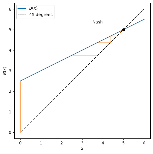
Starting from \(x = 0\) (the Ramsey inflation rate), the government sets \(y = B(0) > 0\).
This provokes the public to raise its expectation, which leads the government to raise inflation further.
The limit of this process is the Nash outcome \(y = x = y^N\), a self-confirming situation.
Thus best response dynamics converge to the Nash equilibrium and reinforce \((U^*, y^N)\) as the prediction of the model without a commitment technology.
85.5. Least squares learning converges to Nash#
A version of the best response dynamics also emerges from least squares learning.
Least squares learning plays a key role throughout this suite of lectures, and this simple example introduces analytical elements that reappear later in more complex settings.
Following [Bray, 1982], assume that expected inflation \(x_t\) is the average of past inflation rates,
which can be represented recursively as
Actual inflation is a disturbed version of the best response mapping evaluated at \(x_t\),
where \(\eta_t\) is an i.i.d. mean-zero term that represents the government’s imperfect control of inflation.
Substituting (85.6) into (85.5) gives the stochastic recursion
By the theory of stochastic approximation, the limiting behavior of \(x_t\) is described by the associated ordinary differential equation (ODE)
The rest point of this ODE satisfies \(x = B(x)\), which is the Nash equilibrium inflation rate \(x = \theta U^*\).
Because the map \(B\) is affine, the ODE is linear with slope
Since \(\mathcal{M} < 0\), the ODE is stable about its rest point, and theorems of [Marcet and Sargent, 1989] give conditions under which \(x_t\) converges to \(y^N\) globally.
Let’s simulate the recursion (85.7) and confirm convergence to the Nash outcome.
def ls_learning(cm, T=2000, σ_η=1.0, seed=0):
    "Simulate least squares learning of expected inflation."
    rng = np.random.default_rng(seed)
    x = np.empty(T + 1)
    y = np.empty(T + 1)
    x[0] = 0.0
    y[0] = cm.B(x[0])
    for t in range(1, T + 1):
        η = σ_η * rng.standard_normal()
        y[t] = cm.B(x[t - 1]) + η
        gain = 1.0 / (t + 1)          # decreasing gain
        x[t] = x[t - 1] + gain * (cm.B(x[t - 1]) - x[t - 1] + η)
    return x, y
x, y = ls_learning(cm, T=2000, σ_η=1.0)

fig, ax = plt.subplots(figsize=(9, 5))
ax.plot(x, 'C0', lw=1, label='expected inflation $x_t$')
ax.axhline(y_N, color='k', ls='--', lw=1, label='Nash $y^N$')
ax.axhline(y_R, color='C2', ls=':', lw=1, label='Ramsey $y^R$')
ax.set_xlabel('$t$')
ax.set_ylabel('inflation')
ax.legend()
plt.show()
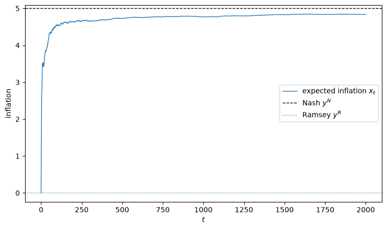
The least squares dynamics confirm the pessimism of the best response dynamics.
Given an initial condition in the form of a low, gold-standard value of \(x\), the best response or least squares dynamics can explain an acceleration of inflation.
But they cannot explain a Volcker-style stabilization that brings inflation back down.
Later lectures reformulate versions of least squares learning in ways designed to moderate this pessimism.
85.6. More foresight#
Best response and least squares learning are out-of-equilibrium dynamics tacked onto a one-period economy.
They force all movement through expectation formation: in choosing inflation, the government forgets that the economy lasts more than one period.
Better outcomes can occur if the government plans for the future.
Subsequent lectures describe three ways of modeling foresight, which impute varying amounts of rationality and predict different qualities of outcomes:
A reputational approach that attributes rational expectations to both the government and the public. Many outcomes are sustainable, ranging from repetition of the Ramsey outcome to paths worse than repetition of the Nash outcome.
An approach that keeps the government rational but gives the public adaptive expectations in the original Cagan-Friedman sense. This is the subject of Adaptive Expectations and the Phelps Problem. Depending on a comparison between a discount factor and an adaptation parameter, this setup can improve outcomes and possibly sustain repetition of the Ramsey outcome.
An approach that attributes adaptive behavior to both the government and the public. This is the subject of Optimal Misspecified Beliefs and Self-Confirming Equilibria.
85.7. Appendix: stochastic approximation#
Here we sketch why the ODE (85.8) governs the tail behavior of the stochastic difference equation (85.7).
The argument, due to [Kushner and Clark, 1978], has two key components: a shift in time scale and a liberal application of averaging.
Let \(\{a_n\}_{n \geq 0}\) be a positive sequence of gains satisfying
The choice \(a_n = 1 / (n + 1)\) satisfies these assumptions.
Rewrite the recursion as
where \(\eta_n\) is i.i.d. with mean zero and finite variance.
Introduce the transformed time scale \(t_0 = 0\), \(t_n = \sum_{i=0}^{n-1} a_i\), and interpolate the discrete sequence \(\{x_n\}\) into a continuous-time process \(x^0(t)\).
Kushner and Clark show that on this transformed time scale the interpolated process is well approximated by the integral equation
where the approximation error \(R(t)\) has two components — one from approximating a distributed lag in \(B(x) - x\) by an integral, and one from a distributed lag in \(\eta_s\).
Studying a sequence of left-shifted versions of the process, they show that both error components can be driven to zero as \(n \to \infty\).
The key step for the noise component is to note that the relevant partial sums form a martingale with variance proportional to \(\sum_i a_i^2\), which converges because \(\sum_i a_i^2 < \infty\).
The remaining error is sent to zero because \(a_i \to 0\) shrinks the mesh of the Riemann sum used to approximate the integral.
In the limit, the stochastic difference equation (85.9) shares the behavior of the non-stochastic ODE
which is said to describe the mean dynamics of the original system.
Later lectures study systems like (85.9) in which \(a_i\) does not approach zero as \(i\) grows — so-called constant gain algorithms.
The mean dynamics (85.8) and these constant-gain algorithms become the central tools of Adaptive Learning and Escape Dynamics, Escaping Nash Inflation, and Priors, Escapes, and Learning Cycles, where the scalar expectation \(x\) studied here grows into a whole vector of drifting Phillips-curve coefficients.
85.8. Exercises#
Exercise 85.1
The convergence rate of least squares learning depends on the slope \(\mathcal{M} = -1/(\theta^2 + 1)\) of the associated ODE.
A necessary condition for convergence at the usual \(\sqrt{t}\) rate is \(\mathcal{M} < -1/2\), which requires \(\theta < 1\).
Simulate least squares learning for \(\theta \in \{0.5, 1.0, 2.0\}\) (holding \(U^*\) fixed) and compare how quickly \(x_t\) settles down near its Nash value \(\theta U^*\).
Plot the three paths of \(x_t - \theta U^*\) on one figure.
Solution
fig, ax = plt.subplots(figsize=(9, 5))

for θ in [0.5, 1.0, 2.0]:
    cm_θ = CredibilityModel(θ=θ, U_star=5.0)
    x, _ = ls_learning(cm_θ, T=3000, σ_η=1.0, seed=1)
    ax.plot(x - cm_θ.nash(), lw=1, label=rf'$\theta = {θ}$')

ax.axhline(0, color='k', lw=0.8)
ax.set_xlabel('$t$')
ax.set_ylabel('$x_t - \\theta U^*$')
ax.legend()
plt.show()
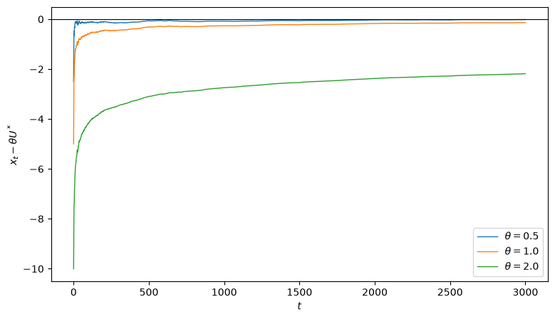
Smaller \(\theta\) (a steeper \(\mathcal{M}\)) produces faster and tighter convergence to the Nash inflation rate.
Larger \(\theta\) leaves \(x_t\) wandering more persistently around its limit.