93. Drifts and Volatilities#
93.1. Overview#
The lectures in this section have told a story about how a government’s model of the Phillips curve, and the policy it induces, can drift over time.
In Adaptive Learning and Escape Dynamics and Escaping Nash Inflation a government that fits and refits an approximating Phillips curve is repeatedly pushed away from a bad self-confirming equilibrium along an escape route, while Priors, Escapes, and Learning Cycles and The Lost Conquest: Fed Policy in the 2020s use drifting beliefs to interpret the rise and fall of American inflation.
Those lectures were mostly about theory.
This lecture turns to the data.
It studies Cogley and Sargent [2005], which asks a deceptively simple question:
When we look at postwar U.S. time series on inflation, unemployment, and interest rates, do we see evidence that the dynamics have drifted?
Tim Cogley and Thomas Sargent began this work as an empirical companion to the Conquest book [Sargent, 1999] and the escape-route papers [Cho et al., 2002].
It is also a response to searching comments by Sims [2001] and Stock [2001] on an earlier paper [Cogley and Sargent, 2001], and it grew into a friendly debate with Sims and Zha [2006] and Bernanke and Mihov [1998] about a question that organizes this whole section:
Was the Great Inflation of the 1970s and its conquest in the 1980s a story of bad policy, or of bad luck?
To let the data speak to that question we need a statistical model flexible enough to accommodate both answers.
That model is a Bayesian vector autoregression whose coefficients drift as random walks and whose shock variances evolve as stochastic volatilities.
Fitting it requires a Markov chain Monte Carlo algorithm that combines the Kalman filter, the forward-filter/backward-sample smoother of Carter and Kohn [1994], and the stochastic-volatility sampler of Jacquier et al. [1994].
Readers who want background will find companion-form vector autoregressions in VARs and DMDs, the Kalman smoother in Another Look at the Kalman Filter, and Bayesian inference for state-space models by MCMC in Posterior Distributions for AR(1) Parameters and Forecasting an AR(1) Process.
We work through the data transformation, prior, sampler, and main empirical results.
Let’s start with some imports and the path to the data.
from pathlib import Path
import time

import matplotlib.pyplot as plt
import numpy as np
import pandas as pd
from IPython.display import display, Math
from scipy import linalg
from scipy.special import expit
from scipy.stats import invwishart


def locate_data_assets():
    """Find assets from either a MyST build or the repository root."""
    relative = Path('_static/lecture_specific/phillips_drifts_volatilities')
    candidates = (relative, Path('lectures') / relative)
    for candidate in candidates:
        if (candidate / 'NEWQDATA.csv').is_file():
            return candidate
    searched = ', '.join(str(path.resolve()) for path in candidates)
    raise FileNotFoundError(f'NEWQDATA.csv was not found; searched {searched}')


asset_path = locate_data_assets()
data_path = asset_path / 'NEWQDATA.csv'
93.2. Bad policy or bad luck?#
Two respectable views compete to explain the American Great Inflation — the same two stories, triumph versus vindication, that open The Rise and Fall of U.S. Inflation.
The bad policy view is the one dramatized throughout this section and in the Conquest book [Sargent, 1999].
Something about Arthur Burns’s model of the economy, his patience, or his inability to commit to a better rule led the Federal Reserve to administer monetary policy in a way that produced the greatest peacetime inflation in U.S. history, while an improved model, more patience, or greater discipline led Paul Volcker to conquer it [DeLong, 1997, Taylor, 1997].
On this view, what changed between the 1970s and the 1980s was the systematic part of policy, namely the way the Fed’s interest-rate setting responded to inflation and unemployment.
The bad luck view says something quite different.
What distinguished the Burns and Volcker eras was not their models or policies, but the shocks that hit the economy.
On this view the coefficients of a reduced-form description of the economy were essentially constant, and what changed was the size of the disturbances, namely the volatility.
Bernanke and Mihov [1998] and Sims and Zha [2006] marshaled evidence for this second view, in part by applying classical tests that failed to reject the hypothesis that VAR coefficients were time invariant.
How can we discriminate?
A constant-coefficient, constant-volatility VAR can generate unusually large realized shocks, but it cannot represent systematic changes in their variance over time.
A model with drifting coefficients but constant volatility can also mistake changing volatility for coefficient drift.
So Cogley and Sargent build a model that has room for both channels at once, and they let a Bayesian posterior sort out how much of each the data call for.
93.3. A VAR with drifting coefficients and stochastic volatility#
Let the variables be ordered as nominal interest, transformed unemployment, and inflation,
(Here \(u_t\) is not the raw unemployment rate but its logit, we define this transformation in the data section below.)
The measurement equation is a VAR with two lags and date-specific coefficients,
Each equation has an intercept and six lag coefficients, so \(\theta_t\) contains \(3(1+2\times 3)=21\) elements.
A two-lag VAR can be rewritten as a one-lag system by stacking \(y_t\) and \(y_{t-1}\) into a single vector; the matrix that multiplies this stacked vector is the companion matrix, and the rewritten system is the VAR in companion form.
The following function builds the companion matrix from the stacked coefficients.
n_variables = 3
n_lags = 2
n_regressors = 1 + n_variables * n_lags
n_coefficients = n_variables * n_regressors


def companion_matrix(θ):
    """Return the intercept and companion matrix for one coefficient vector."""
    equation_rows = np.asarray(θ, dtype=float).reshape(
        n_variables, n_regressors
    )
    intercept = np.r_[equation_rows[:, 0], np.zeros(n_variables)]
    companion = np.zeros((n_variables * n_lags, n_variables * n_lags))
    companion[:n_variables] = equation_rows[:, 1:]
    companion[n_variables:, :n_variables] = np.eye(n_variables)
    return intercept, companion


def design_matrix(regressors):
    """Return the observation matrix X_t prime for one date."""
    return np.kron(np.eye(n_variables), np.asarray(regressors, dtype=float))
The coefficient vector follows a driftless random walk,
A prior over how fast coefficients drift plays a mirror-image role in Priors, Escapes, and Learning Cycles: there it is the government’s prior about a drifting Phillips curve that shapes the policy it chooses, whereas here it is the econometrician’s prior in a posterior about drifting reduced-form dynamics.
The companion system is stable when every companion-matrix eigenvalue lies strictly inside the unit circle.
For an AR(1), this is \(|\rho|<1\); equivalently, the zero of \(1-\rho z\) lies outside the unit circle.
Cogley and Sargent rule out explosive paths by retaining a path only when the companion matrix is stable at every date and using the truncated prior
where \(I(\theta^T)=1\) denotes a stable path.
This restriction encodes the belief that the economy did not in fact follow an explosive path.
This restriction also tilts the marginal prior for \(Q\) toward values that are less likely to generate explosive coefficient paths.
The code below applies the stability restriction to an entire trajectory
def companion_roots(θ_path):
    """Return all companion roots along a path with shape (21, T)."""
    θ_path = np.asarray(θ_path, dtype=float)
    if θ_path.ndim == 1:
        θ_path = θ_path[:, None]
    companions = np.stack(
        [
            companion_matrix(θ_path[:, t])[1]
            for t in range(θ_path.shape[1])
        ]
    )
    return np.linalg.eigvals(companions)


def is_stable(θ_path):
    """Test whether every companion root is strictly inside the unit circle."""
    return bool(np.max(np.abs(companion_roots(θ_path))) < 1)
The reduced-form innovation covariance changes over time according to
where
The diagonal elements \(h_{it}\) let the size of each orthogonalized shock wax and wane over time.
The next two functions construct the triangular factor and the reduced-form innovation covariance.
def b_matrix(β):
    """Construct B from β_21, β_31, and β_32."""
    matrix = np.eye(n_variables)
    matrix[1, 0], matrix[2, 0], matrix[2, 1] = np.asarray(β, dtype=float)
    return matrix


def innovation_covariance(h, β):
    """Construct R_t from one vector of orthogonalized variances."""
    inverse = np.linalg.inv(b_matrix(β))
    return inverse @ np.diag(h) @ inverse.T
Each diagonal volatility is a geometric random walk,
The standardized measurement innovations, coefficient innovations, and volatility innovations are mutually independent.
Setting \(Q=0\) produces constant coefficients with drifting volatility, while holding \(H_t\) fixed produces drifting coefficients with constant volatility.
The posterior contains the full paths \(\theta^T\) and \(H^T\) together with \(Q\), \(\beta\), and \((\sigma_1,\sigma_2,\sigma_3)\).
This posterior has thousands of dimensions, so later sections build a sampler that updates one group of parameters at a time, holding the rest fixed.
93.4. The data#
We begin with Cogley and Sargent [2005]’s quarterly U.S. dataset ending in 2000Q4.
Inflation is the log difference of the seasonally adjusted CPI for all urban consumers, point sampled in the third month of each quarter.
Unemployment is the quarterly average of the seasonally adjusted civilian unemployment rate and enters the VAR as \(0.01\log[u/(1-u)]\), a logit transformation that maps a bounded rate into an unconstrained variable.
The nominal interest rate is the log of one plus the three-month Treasury-bill rate, averaged over daily observations in the first month of each quarter and expressed as a quarterly fraction.
The data starts in 1948Q2 because its first inflation observation is already differenced, so two VAR lags make 1948Q4 the first usable regression date.
The following cell performs every transformation and constructs the VAR(2) data directly from the series.
def prepare_data(source, ordering=('i', 'u', 'pi')):
    """Transform a quarterly table and construct the VAR data."""
    if isinstance(source, (str, Path)):
        table = pd.read_csv(source)
    else:
        table = source.copy()
    variables = {
        'i': table['y3'].to_numpy(dtype=float),
        'u': 0.01 * np.log(
            table['ur'].to_numpy(dtype=float)
            / (1 - table['ur'].to_numpy(dtype=float))
        ),
        'pi': table['dp'].to_numpy(dtype=float),
    }
    if sorted(ordering) != ['i', 'pi', 'u']:
        raise ValueError("ordering must be a permutation of ('i', 'u', 'pi')")
    raw_y = np.column_stack([variables[name] for name in ordering])
    raw_dates = table['date'].to_numpy(dtype=float)
    regressors = np.ones((len(table) - n_lags, n_regressors))
    for lag in range(1, n_lags + 1):
        left = 1 + n_variables * (lag - 1)
        regressors[:, left:left + n_variables] = raw_y[n_lags-lag:-lag]
    targets = raw_y[n_lags:]
    dates = raw_dates[n_lags:]
    n_training = 4 * 11 - n_lags - 1
    return {
        'raw_dates': raw_dates,
        'raw_y': raw_y,
        'prior_dates': dates[:n_training],
        'prior_y': targets[:n_training],
        'prior_x': regressors[:n_training],
        'dates': dates[n_training:],
        'y': targets[n_training:],
        'x': regressors[n_training:],
    }


data = prepare_data(data_path)

data_summary = pd.Series(
    {
        'ordering': 'interest, unemployment, inflation',
        'prior sample': '1948Q4--1958Q4',
        'prior observations': len(data['prior_dates']),
        'posterior sample': '1959Q1--2000Q4',
        'posterior observations': len(data['dates']),
        'VAR lags': n_lags,
        'coefficient dimension': n_coefficients,
    },
    name='value',
)

data_summary.to_frame()
| value | |
|---|---|
| ordering | interest, unemployment, inflation |
| prior sample | 1948Q4--1958Q4 |
| prior observations | 41 |
| posterior sample | 1959Q1--2000Q4 |
| posterior observations | 168 |
| VAR lags | 2 |
| coefficient dimension | 21 |
The early observations calibrate the prior, while the remaining observations form the posterior sample.
Let’s view the data in familiar economic units.
dates_raw = data['raw_dates']
interest = 400 * np.expm1(data['raw_y'][:, 0])
unemployment = 100 * expit(100 * data['raw_y'][:, 1])
inflation = 400 * data['raw_y'][:, 2]

fig, axes = plt.subplots(3, 1, figsize=(9, 7), sharex=True)
axes[0].plot(dates_raw, inflation, lw=2)
axes[0].set_ylabel('inflation (annual %)')
axes[1].plot(dates_raw, unemployment, lw=2)
axes[1].set_ylabel('unemployment (%)')
axes[2].plot(dates_raw, interest, lw=2)
axes[2].set_ylabel('interest (annual %)')
axes[2].set_xlabel('year')
plt.tight_layout()
plt.show()
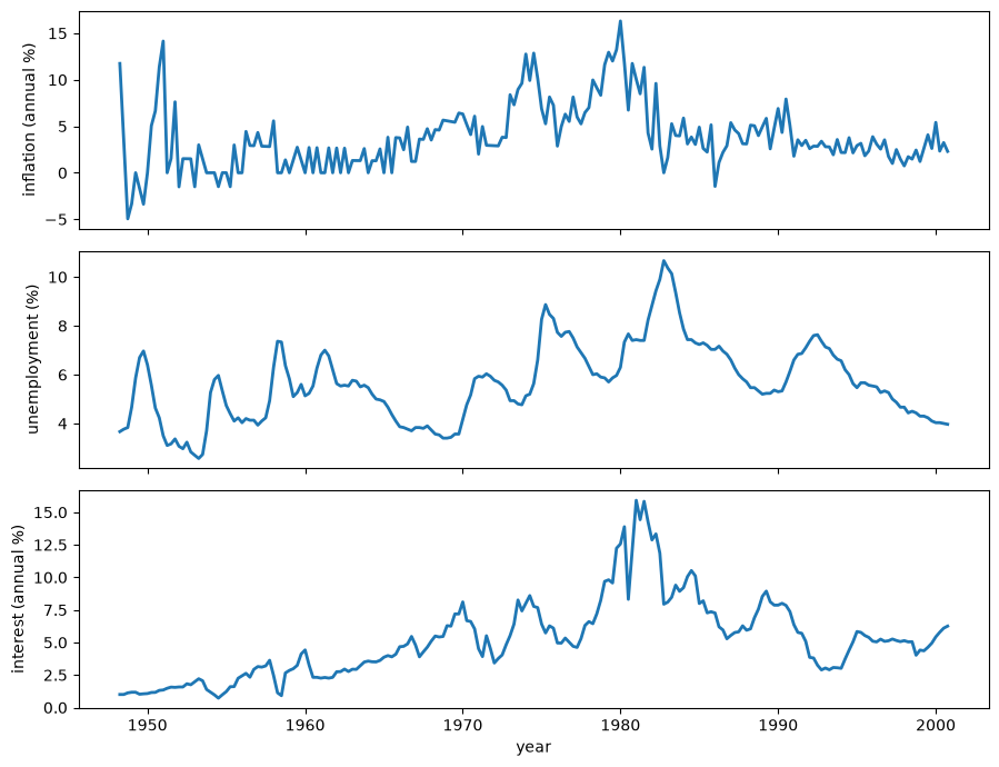
Fig. 93.1 Observed \(\pi_t\), \(u_t\), and \(i_t\), 1948Q2–2000Q4#
Inflation and nominal interest rates rise together through the 1970s and peak around 1980, unemployment peaks only after disinflation begins, and all three series are calmer in the 1990s.
These observations locate the episode but cannot tell whether changed systematic dynamics or unusually large shocks produced it, which is the distinction the model is built to examine.
93.5. Priors#
The priors are independent across parameters and deliberately weak so that, in Cogley and Sargent’s phrase, “the data are free to speak.”
They are calibrated from a time-invariant VAR fitted to the short 1948–1958 training sample.
The initial coefficient prior is a stable, truncated Gaussian,
where \(\bar\theta\) and \(\bar P\) come from a constant-coefficient seemingly unrelated regression fitted to the 1948–1958 training sample.
Because all three equations have identical regressors, the SUR coefficient estimates equal equation-by-equation OLS estimates, which lets us implement the calibration compactly.
def sur_prior(y, x):
    """Calibrate the Gaussian coefficient prior from a constant VAR."""
    xx_inverse = np.linalg.inv(x.T @ x)
    coefficients = xx_inverse @ x.T @ y
    residuals = y - x @ coefficients
    residual_covariance = np.cov(residuals, rowvar=False, ddof=1)
    θ = coefficients.T.reshape(-1)
    covariance = np.kron(residual_covariance, xx_inverse)
    return θ, covariance, residual_covariance


θ_bar, p_bar, r_bar = sur_prior(data['prior_y'], data['prior_x'])

assert is_stable(θ_bar)
The coefficient-drift covariance has the inverse-Wishart prior
The convention in (93.6) lists degrees of freedom first and the inverse-Wishart scale matrix second.
Because \(T_0\) is only one greater than the dimension of \(\theta_t\), the prior is proper but has no finite mean.
The matrix \(\bar Q\) is therefore a conservative scale calibration rather than the expectation of \(Q\).
This calibration favors slow coefficient drift before the posterior sees the main sample.
The remaining priors are
where \(\bar R\) is the residual covariance from the training-sample regression.
The next function gathers these hyperparameters.
def calibrate_prior(model_data, γ_squared=3.5e-4):
    """Return every calibrated prior for one variable ordering."""
    θ_mean, θ_covariance, residual_covariance = sur_prior(
        model_data['prior_y'], model_data['prior_x']
    )
    degrees_freedom = n_coefficients + 1
    q_center = γ_squared * θ_covariance
    return {
        'θ_mean': θ_mean,
        'θ_covariance': θ_covariance,
        'q_center': q_center,
        'q_scale': degrees_freedom * q_center,
        'q_degrees_freedom': degrees_freedom,
        'log_h_mean': np.log(np.diag(residual_covariance)),
        'log_h_variance': 10.0,
        'β_mean': np.zeros(3),
        'β_variance': 10000.0,
        'σ_degrees_freedom': 1.0,
        'σ_scale': 0.01**2,
        'γ_squared': γ_squared,
    }


prior = calibrate_prior(data)
q_bar = prior['q_center']

prior_summary = pd.Series(
    {
        'dim(θ)': n_coefficients,
        'T0': prior['q_degrees_freedom'],
        'γ squared': prior['γ_squared'],
        'trace(Q bar)': np.trace(q_bar),
        'log-h prior variance': prior['log_h_variance'],
        'β prior variance': prior['β_variance'],
        'σ-squared IG shape': prior['σ_degrees_freedom'] / 2,
        'σ-squared IG scale': prior['σ_scale'] / 2,
    },
    name='value',
)

prior_summary.to_frame()
| value | |
|---|---|
| dim(θ) | 21.000000 |
| T0 | 22.000000 |
| γ squared | 0.000350 |
| trace(Q bar) | 0.003004 |
| log-h prior variance | 10.000000 |
| β prior variance | 10000.000000 |
| σ-squared IG shape | 0.500000 |
| σ-squared IG scale | 0.000050 |
93.6. A Metropolis-within-Gibbs sampler#
We simulate the posterior by cycling through five parameter blocks used by Cogley and Sargent [2005].
One pass through all five blocks is called a sweep, and the sampler runs many sweeps to build up the posterior sample.
Cogley and Sargent simulate the unrestricted posterior and then discard a complete MCMC realization whenever its coefficient path is explosive.
But in this case only stable sweeps contribute realizations to the retained restricted-posterior sample.
We instead impose stability inside the coefficient-path block with the elliptical slice sampler of Murray et al. [2010].
This changes the transition kernel, but not its target posterior.
An auxiliary Gaussian coefficient path is drawn by a Carter–Kohn forward-filter/backward-sample step and used to update the stable path by elliptical slice sampling.
The drift covariance \(Q\) is drawn from an inverse-Wishart distribution conditional on the coefficient innovations.
The volatility innovation variances \(\sigma_i^2\) are drawn from inverse-gamma distributions conditional on the volatility increments.
The covariance parameters \(\beta\) are drawn from two transformed Gaussian regressions among the VAR residuals.
The volatility paths \(H^T\) are drawn one date at a time by a Jacquier–Polson–Rossi Metropolis step.
This ordering matters: every block in a sweep is paired with the values on which it was actually conditioned.
93.6.1. Coefficient path#
Conditional on \(R^T\) and \(Q\), a forward Kalman filter followed by the Carter–Kohn backward simulator draws the entire coefficient path [Carter and Kohn, 1994].
The forward pass is a Kalman filter, while the backward pass samples \(\theta_T,\theta_{T-1},\ldots,\theta_0\) in reverse with each state conditioned on the draw that follows it.
Sampling \(\theta_0\) is essential.
It supplies all \(T\) random-walk increments to the conjugate update for \(Q\).
def covariance_root(matrix):
    """Return a numerically stable lower covariance factor."""
    matrix = 0.5 * (matrix + matrix.T)
    scale = max(1.0, np.max(np.abs(np.diag(matrix))))
    return np.linalg.cholesky(matrix + 1e-12 * scale * np.eye(len(matrix)))


def draw_coefficient_path(
    y, x, q, h, β, prior, rng, return_mean=False
):
    """Draw θ_0,...,θ_T and optionally return its smoothing mean."""
    periods = len(y)
    filtered_mean = np.empty((periods + 1, n_coefficients))
    filtered_covariance = np.empty(
        (periods + 1, n_coefficients, n_coefficients)
    )
    predicted_covariance = np.empty_like(filtered_covariance)
    filtered_mean[0] = prior['θ_mean']
    filtered_covariance[0] = prior['θ_covariance']
    predicted_covariance[0] = prior['θ_covariance']
    for t in range(1, periods + 1):
        observation = design_matrix(x[t - 1])
        prediction_covariance = filtered_covariance[t - 1] + q
        r_t = innovation_covariance(h[t], β)
        forecast_covariance = (
            observation @ prediction_covariance @ observation.T + r_t
        )
        gain = linalg.solve(
            forecast_covariance,
            (prediction_covariance @ observation.T).T,
            assume_a='pos',
        ).T
        mean = filtered_mean[t - 1]
        mean = mean + gain @ (y[t - 1] - observation @ mean)
        covariance = (
            prediction_covariance
            - gain @ observation @ prediction_covariance
        )
        covariance = 0.5 * (covariance + covariance.T)
        filtered_mean[t] = mean
        filtered_covariance[t] = covariance
        predicted_covariance[t] = prediction_covariance
    path = np.empty((n_coefficients, periods + 1))
    if not return_mean:
        path[:, -1] = (
            filtered_mean[-1]
            + covariance_root(filtered_covariance[-1])
            @ rng.standard_normal(n_coefficients)
        )
        for t in range(periods - 1, -1, -1):
            smoother = linalg.solve(
                predicted_covariance[t + 1],
                filtered_covariance[t].T,
                assume_a='pos',
            ).T
            mean = filtered_mean[t] + smoother @ (
                path[:, t + 1] - filtered_mean[t]
            )
            covariance = (
                filtered_covariance[t]
                - smoother @ predicted_covariance[t + 1] @ smoother.T
            )
            path[:, t] = mean + covariance_root(covariance) @ (
                rng.standard_normal(n_coefficients)
            )
        return path

    smoothed_mean = np.empty_like(path)
    centered_draw = np.empty_like(path)
    smoothed_mean[:, -1] = filtered_mean[-1]
    centered_draw[:, -1] = covariance_root(filtered_covariance[-1]) @ (
        rng.standard_normal(n_coefficients)
    )
    for t in range(periods - 1, -1, -1):
        smoother = linalg.solve(
            predicted_covariance[t + 1],
            filtered_covariance[t].T,
            assume_a='pos',
        ).T
        smoothed_mean[:, t] = filtered_mean[t] + smoother @ (
            smoothed_mean[:, t + 1] - filtered_mean[t]
        )
        covariance = (
            filtered_covariance[t]
            - smoother @ predicted_covariance[t + 1] @ smoother.T
        )
        centered_draw[:, t] = (
            smoother @ centered_draw[:, t + 1]
            + covariance_root(covariance) @ rng.standard_normal(n_coefficients)
        )
    return smoothed_mean + centered_draw, smoothed_mean


def draw_stable_coefficient_path(
    current, y, x, q, h, β, prior, rng, max_contractions=100
):
    """Elliptical-slice update of the stability-truncated Gaussian path."""
    if not is_stable(current):
        raise ValueError('the elliptical-slice update needs a stable path')
    gaussian_draw, mean = draw_coefficient_path(
        y, x, q, h, β, prior, rng, return_mean=True
    )
    current_centered = current - mean
    innovation = gaussian_draw - mean
    angle = rng.uniform(0, 2 * np.pi)
    lower = angle - 2 * np.pi
    upper = angle
    for contractions in range(max_contractions + 1):
        proposal = (
            mean
            + current_centered * np.cos(angle)
            + innovation * np.sin(angle)
        )
        if is_stable(proposal):
            return proposal, contractions
        if angle < 0:
            lower = angle
        else:
            upper = angle
        angle = rng.uniform(lower, upper)
    raise RuntimeError('elliptical-slice stability bracket did not contract')
93.6.2. Drift covariance#
Conditional on the coefficient increments, \(Q\) has an inverse-Wishart full conditional.
The retained simulation draws \(Q\) from a scale matrix formed by its prior scale and all \(T\) squared increments from \(\theta_0\) through \(\theta_T\).
def draw_q(θ_path, prior, rng):
    """Draw Q conditional on the sampled coefficient path."""
    increments = np.diff(θ_path, axis=1)
    scale = prior['q_scale'] + increments @ increments.T
    degrees_freedom = prior['q_degrees_freedom'] + increments.shape[1]
    return invwishart.rvs(df=degrees_freedom, scale=scale, random_state=rng)
93.6.3. Volatility parameters and paths#
Conditional on the volatility increments, each \(\sigma_i^2\) has an inverse-gamma full conditional.
Conditional on the VAR residuals and \(H^T\), the free elements of \(B\) are drawn from two Gaussian regressions.
Conditional on the orthogonalized residuals, each volatility state is updated with the single-site Metropolis step of Jacquier et al. [1994].
The random-walk neighbors determine the Gaussian proposal for a log volatility, while the corresponding orthogonalized residual determines whether that proposal is accepted.
The following code implements the conditional updates, including the different endpoint proposals.
def var_residuals(y, x, θ_path):
    """Return residuals with shape (T, 3)."""
    if θ_path.shape[1] == len(y) + 1:
        θ_path = θ_path[:, 1:]
    if θ_path.shape[1] != len(y):
        raise ValueError('θ_path must contain T or T + 1 states')
    coefficients = θ_path.T.reshape(len(y), n_variables, n_regressors)
    fitted = np.einsum('tk,tnk->tn', x, coefficients)
    return y - fitted


def draw_σ(h, prior, rng):
    """Draw the three log-volatility innovation standard deviations."""
    increments = np.diff(np.log(h), axis=0)
    shape = (prior['σ_degrees_freedom'] + increments.shape[0]) / 2
    scales = (prior['σ_scale'] + np.sum(increments**2, axis=0)) / 2
    σ_squared = scales / rng.gamma(shape, 1.0, size=n_variables)
    return np.sqrt(σ_squared)


def draw_β(residuals, h, prior, rng):
    """Draw the free elements of B from transformed Gaussian regressions."""
    β = np.empty(3)
    offset = 0
    for equation in range(1, n_variables):
        standardized = residuals / np.sqrt(h[1:, equation])[:, None]
        dependent = standardized[:, equation]
        regressors = -standardized[:, :equation]
        prior_precision = np.eye(equation) / prior['β_variance']
        covariance = np.linalg.inv(prior_precision + regressors.T @ regressors)
        prior_slice = prior['β_mean'][offset:offset + equation]
        mean = covariance @ (
            prior_precision @ prior_slice + regressors.T @ dependent
        )
        β[offset:offset + equation] = (
            mean + covariance_root(covariance) @ rng.standard_normal(equation)
        )
        offset += equation
    return β


def accept_volatility(proposal, current, residual, rng):
    """Apply the Jacquier--Polson--Rossi likelihood acceptance step."""
    log_ratio = (
        -0.5 * np.log(proposal)
        - residual**2 / (2 * proposal)
        + 0.5 * np.log(current)
        + residual**2 / (2 * current)
    )
    return proposal if np.log(rng.random()) <= min(0.0, log_ratio) else current


def draw_volatility_path(h, residuals, β, σ, prior, rng):
    """Update all stochastic-volatility states one date at a time."""
    periods = len(residuals)
    orthogonalized = (b_matrix(β) @ residuals.T).T
    updated = np.empty_like(h)
    for equation in range(n_variables):
        variance = σ[equation]**2
        initial_variance = (
            prior['log_h_variance'] * variance
            / (variance + prior['log_h_variance'])
        )
        initial_mean = initial_variance * (
            prior['log_h_mean'][equation] / prior['log_h_variance']
            + np.log(h[1, equation]) / variance
        )
        updated[0, equation] = np.exp(
            initial_mean + np.sqrt(initial_variance) * rng.standard_normal()
        )
        for t in range(1, periods):
            mean = 0.5 * (
                np.log(updated[t - 1, equation]) + np.log(h[t + 1, equation])
            )
            proposal = np.exp(
                mean + np.sqrt(variance / 2) * rng.standard_normal()
            )
            updated[t, equation] = accept_volatility(
                proposal,
                h[t, equation],
                orthogonalized[t - 1, equation],
                rng,
            )
        proposal = np.exp(
            np.log(updated[-2, equation])
            + σ[equation] * rng.standard_normal()
        )
        updated[-1, equation] = accept_volatility(
            proposal,
            h[-1, equation],
            orthogonalized[-1, equation],
            rng,
        )
    return updated
93.6.4. Complete sampler#
The restricted posterior assigns zero density to coefficient paths that are explosive at any date, including \(\theta_0\).
Stack the whole coefficient path \(\theta_0,\ldots,\theta_T\) into \(z\), and collect the other parameter blocks in \(\lambda=(Q,H^T,\beta,\sigma)\).
Conditional on \(\lambda\) and the data \(Y^T\), the unrestricted Carter–Kohn distribution is Gaussian with smoothing mean \(m\) and covariance \(C\),
Let \(\mathcal A\) be the set of paths whose companion roots are strictly inside the unit circle at every date, so that the restricted full conditional is this Gaussian truncated to \(\mathcal A\),
That normalizing probability is difficult to compute, but the elliptical transition never evaluates it.
Cogley and Sargent instead simulate the unrestricted joint posterior and keep a realization only when its whole path is stable, which is valid because conditioning the unrestricted posterior on \(z\in\mathcal A\) reproduces the restricted posterior exactly.
If \(a\) denotes the unrestricted probability that a path is stable, this rejection scheme needs roughly \(1/a\) complete sweeps, including the four other parameter updates, for every retained draw.
The elliptical slice sampler avoids that waste by moving within the stable region instead of restarting from an arbitrary draw.
It starts from the current stable path \(z^{(c)}\) and a fresh Carter–Kohn draw \(\widetilde z\sim N(m,C)\), whose centered version \(\nu=\widetilde z-m\) traces an ellipse together with \(z^{(c)}\),
so that \(z(0)=z^{(c)}\) and \(z(\pi/2)=\widetilde z\).
The algorithm draws an angle uniformly from the full circle and, whenever \(z(\phi)\) is explosive, shrinks the bracket to the side containing the known-stable angle \(\phi=0\) before drawing again.
Because companion roots vary continuously with the coefficients, a nonzero interval around \(\phi=0\) is always stable, so this bracket search always terminates.
Each rejected angle costs only a linear combination and a companion-root check, far cheaper than another Kalman filter and backward simulation.
The transition is valid because rotating the pair \((z^{(c)}-m,\nu)\) by any angle leaves their joint Gaussian density unchanged, so the search moves along a fixed orbit on which every point is equally likely under the unrestricted density.
The stability indicator plays the role of the likelihood in a standard elliptical slice update, and since it equals one at the current point, every accepted angle is automatically a stable one and no separate slice-height draw is needed.
Marginalizing out the auxiliary path shows that this transition leaves the truncated Gaussian \(N(z;m,C)\mathbb{1}_{\mathcal A}(z)\) invariant, exactly the property a valid transition kernel needs.
The other four blocks require no such adjustment.
Conditional on a stable \(z\), the stability indicator is constant in \(Q,H^T,\beta\), and \(\sigma\), so it cancels from each of their full conditionals and leaves the same updates as the unrestricted sampler.
\(Q\)’s conditional is unchanged in form, but its marginal posterior still tilts toward less explosive drift because every draw of \(Q\) is conditioned on a stable coefficient path.
Together, the elliptical transition for \(z\) and the unchanged updates for \(Q,H^T,\beta\), and \(\sigma\) target the same stability-restricted posterior as Cogley and Sargent’s original rejection sampler, at a fraction of the cost.
The next function composes these five blocks and includes a stochastic-volatility warm-up.
def initial_volatilities(y, prior):
    """Construct the sampler's initial volatility path."""
    changes = np.diff(y, axis=0)
    centered = changes - changes.mean(axis=0)
    log_h = np.empty((len(y) + 1, n_variables))
    log_h[:2] = prior['log_h_mean']
    log_h[2:] = np.log(np.maximum(centered**2, np.finfo(float).tiny))
    return np.exp(log_h)


def run_sampler(
    y,
    x,
    prior,
    n_sweeps=1_000,
    burn=500,
    thin=1,
    seed=42,
    warmup=200,
    max_contractions=100,
    stable=True,
    fixed_q=None,
    retain=('S0D', 'SD', 'QD', 'HD', 'CD', 'VD', 'stable_draw'),
    progress_every=0,
):
    """Run a Gibbs sampler for the unrestricted or stable posterior.

    For the stable posterior, an elliptical-slice transition updates the FFBS
    path inside its stability-truncated Gaussian full conditional.  Passing
    ``fixed_q`` holds Q at that value (for example a matrix of zeros) instead of
    drawing it, which nests the constant-coefficient model.
    """
    if not (0 <= burn < n_sweeps and thin >= 1):
        raise ValueError('require 0 <= burn < n_sweeps and thin >= 1')
    if (n_sweeps - burn) % thin:
        raise ValueError('(n_sweeps - burn) must be divisible by thin')
    valid_retain = {'S0D', 'SD', 'QD', 'HD', 'CD', 'VD', 'stable_draw'}
    unknown = set(retain) - valid_retain
    if unknown:
        raise ValueError(f'unknown retained arrays: {sorted(unknown)}')

    started = time.perf_counter()
    rng = np.random.default_rng(seed)
    h = initial_volatilities(y, prior)
    β = prior['β_mean'].copy()
    warm_θ = np.repeat(prior['θ_mean'][:, None], len(y), axis=1)
    warm_residuals = var_residuals(y, x, warm_θ)
    for _ in range(warmup):
        σ = draw_σ(h, prior, rng)
        β = draw_β(warm_residuals, h, prior, rng)
        h = draw_volatility_path(
            h, warm_residuals, β, σ, prior, rng
        )

    q = (
        prior['q_center'].copy()
        if fixed_q is None
        else np.array(fixed_q, dtype=float)
    )
    θ = np.repeat(
        prior['θ_mean'][:, None], len(y) + 1, axis=1
    )
    if stable and not is_stable(θ):
        raise ValueError('the prior mean does not provide a stable start')
    slice_contractions = 0
    maximum_slice_contractions = 0

    retained = {name: [] for name in retain}
    saved_stability = []
    for sweep in range(1, n_sweeps + 1):
        if stable:
            θ, contractions = draw_stable_coefficient_path(
                θ,
                y,
                x,
                q,
                h,
                β,
                prior,
                rng,
                max_contractions=max_contractions,
            )
        else:
            θ = draw_coefficient_path(y, x, q, h, β, prior, rng)
            contractions = 0
        slice_contractions += contractions
        maximum_slice_contractions = max(
            maximum_slice_contractions, contractions
        )
        if fixed_q is None:
            q = draw_q(θ, prior, rng)
        residuals = var_residuals(y, x, θ)
        σ = draw_σ(h, prior, rng)
        β = draw_β(residuals, h, prior, rng)
        h = draw_volatility_path(
            h, residuals, β, σ, prior, rng
        )

        if sweep > burn and (sweep - burn) % thin == 0:
            path_is_stable = is_stable(θ)
            saved_stability.append(path_is_stable)
            values = {
                'S0D': θ[:, 0],
                'SD': θ[:, 1:],
                'QD': q,
                'HD': h,
                'CD': β,
                'VD': σ,
                'stable_draw': path_is_stable,
            }
            for name in retained:
                retained[name].append(np.asarray(values[name]).copy())

        if progress_every and sweep % progress_every == 0:
            elapsed = time.perf_counter() - started
            print(
                f'{sweep:,}/{n_sweeps:,} sweeps; '
                f'{slice_contractions:,} slice contractions; '
                f'{elapsed / 60:.1f} minutes',
                flush=True,
            )

    stack_axis = {
        'S0D': 1,
        'SD': 2,
        'QD': 2,
        'HD': 2,
        'CD': 1,
        'VD': 1,
        'stable_draw': 0,
    }
    result = {
        name: np.stack(values, axis=stack_axis[name])
        for name, values in retained.items()
    }
    result['diagnostics'] = {
        'sampler_version': 3,
        'seed': int(seed),
        'stable_restriction': bool(stable),
        'n_sweeps': int(n_sweeps),
        'burn': int(burn),
        'thin': int(thin),
        'warmup': int(warmup),
        'retained_draws': int((n_sweeps - burn) // thin),
        'slice_contractions': int(slice_contractions),
        'mean_slice_contractions': float(slice_contractions / n_sweeps),
        'maximum_slice_contractions': int(maximum_slice_contractions),
        'retained_stability_rate': float(np.mean(saved_stability)),
        'elapsed_seconds': float(time.perf_counter() - started),
    }
    return result
The executable version below uses 1,000 sweeps, discards the first 500, and retains the remaining 500.
It uses the complete historical sample and the ordering \((i,u,\pi)\).
Instead of running a large MCMC experiment, we intentionally keep the sampler run small so that it finishes in a reasonable time for a lecture.
This short run illustrates the method but not a numerical replication.
However the main qualitative features of the posterior are close to those reported by Cogley and Sargent.
posterior = run_sampler(
    data['y'],
    data['x'],
    prior,
    n_sweeps=1_000,
    burn=500,
    thin=1,
    seed=42,
    warmup=200,
    stable=True,
    progress_every=0,
)

def validate_posterior_arrays(result, periods):
    """Check posterior shapes, finiteness, positivity, and stability."""
    draws = result['diagnostics']['retained_draws']
    expected = {
        'S0D': (n_coefficients, draws),
        'SD': (n_coefficients, periods, draws),
        'QD': (n_coefficients, n_coefficients, draws),
        'HD': (periods + 1, n_variables, draws),
        'CD': (3, draws),
        'VD': (3, draws),
        'stable_draw': (draws,),
    }
    assert {name: result[name].shape for name in expected} == expected
    assert all(np.all(np.isfinite(result[name])) for name in expected)
    assert np.all(result['HD'] > 0)
    assert np.all(result['VD'] > 0)
    assert np.all(result['stable_draw'])
    return expected


expected_shapes = validate_posterior_arrays(posterior, len(data['dates']))
93.7. What the data say#
We summarize the posterior by its mean coefficient path \(E(\theta_t\mid T)\) and mean covariance path \(E(R_t\mid T)\), and then interpret them in the context of the question we asked.
93.7.1. The rate and structure of drift#
The trace of \(Q\) measures the total rate of coefficient drift, with \(\operatorname{tr}(Q)=0\) corresponding to constant coefficients.
The histogram shows the retained \(Q\) draws and the prior scale.
trace_q = np.trace(posterior['QD'], axis1=0, axis2=1)
fig, ax = plt.subplots()
ax.hist(trace_q, bins=30, histtype='step', lw=2)
ax.axvline(np.trace(q_bar), color='C1', lw=2,
           label=r'prior $\mathrm{tr}(\bar Q)$')
ax.set_xlabel(r'$\mathrm{tr}(Q)$')
ax.set_ylabel('frequency')
ax.legend()
plt.show()
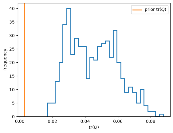
Fig. 93.2 Posterior \(\operatorname{tr}(Q)\) and prior \(\operatorname{tr}(\bar Q)\)#
The posterior drift rate lies well above the conservative prior calibration, indicating more coefficient variation than that calibration anticipated.
This is not a formal comparison with a fixed-coefficient model because the continuous prior assigns no point mass to \(Q=0\).
Within the fitted TVP-VAR, this variation is attributed to changing systematic relationships; it does not identify policy as the cause.
θ_mean = posterior['SD'].mean(axis=2)
mean_path_root_modulus = np.max(
    np.abs(companion_roots(θ_mean)), axis=1
)
assert np.all(mean_path_root_modulus < 1)
coefficient_labels = (
    'constant',
    r'$i_{t-1}$',
    r'$u_{t-1}$',
    r'$\pi_{t-1}$',
    r'$i_{t-2}$',
    r'$u_{t-2}$',
    r'$\pi_{t-2}$',
)
equation_labels = (
    'interest equation',
    'unemployment equation',
    'inflation equation',
)


def plot_equation_coefficients(axes, dates, θ_path):
    """Plot seven labeled coefficients for each VAR equation."""
    first_lines = None
    for equation, (ax, label) in enumerate(zip(axes, equation_labels)):
        start = equation * len(coefficient_labels)
        stop = start + len(coefficient_labels)
        lines = ax.plot(dates, θ_path[start:stop].T, lw=2)
        for line, coefficient_label in zip(lines, coefficient_labels):
            line.set_label(coefficient_label)
        if first_lines is None:
            first_lines = lines
        ax.axhline(0, color='0.65', lw=1)
        ax.set_xlabel('year')
        ax.set_ylabel(f'{label} coefficient')
    return first_lines


fig, axes = plt.subplots(1, 3, figsize=(10, 4), sharex=True)
coefficient_lines = plot_equation_coefficients(
    axes,
    data['dates'],
    θ_mean,
)
fig.legend(
    coefficient_lines,
    coefficient_labels,
    loc='lower center',
    ncol=4,
)
plt.tight_layout(rect=(0, 0.17, 1, 1))
plt.show()
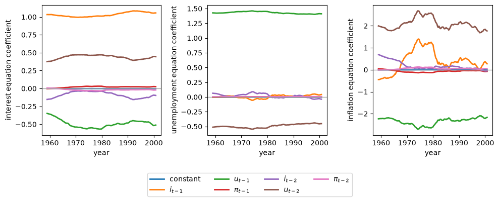
Fig. 93.3 Posterior mean VAR coefficients \(E(\theta_t\mid T)\)#
The unemployment equation is comparatively stable, whereas several inflation equation coefficients move strongly through the 1970s and turn around near 1980.
The drift is therefore concentrated in how inflation propagates rather than spread evenly across the VAR, and individual lag coefficients should not be given structural interpretations because paired lags can offset one another.
We summarize drift for the ordering \((i,u,\pi)\), which has the smallest stable posterior mean \(\operatorname{tr}(Q)\).
trace_q = np.trace(posterior['QD'], axis1=0, axis2=1)
q_mean = posterior['QD'].mean(axis=2)
drift_summary = {
    r'\text{Posterior mean } \operatorname{tr}(Q)': np.trace(q_mean),
    r'\text{Posterior mean largest eigenvalue}': (
        np.linalg.eigvalsh(q_mean)[-1]
    ),
    r'\text{Prior } \operatorname{tr}(\bar Q)': np.trace(q_bar),
}
drift_rows = ' \\\\\n'.join(
    f'{label} & {value:.4f}' for label, value in drift_summary.items()
)
display(Math(rf'''
\begin{{array}}{{lr}}
\text{{Quantity}} & \text{{Estimate}} \\
\hline
{drift_rows}
\end{{array}}
'''))
Cogley and Sargent estimated every ordering.
Their posterior means show that the ordering changes magnitudes but does not remove drift:
Ordering |
Stable \(\operatorname{tr}(Q)\) |
Stable \(\max(\lambda)\) |
Unrestricted \(\operatorname{tr}(Q)\) |
Unrestricted \(\max(\lambda)\) |
|---|---|---|---|---|
\((i,\pi,u)\) |
0.055 |
0.025 |
0.056 |
0.027 |
\((i,u,\pi)\) |
0.047 |
0.023 |
0.059 |
0.031 |
\((\pi,i,u)\) |
0.064 |
0.031 |
0.082 |
0.044 |
\((\pi,u,i)\) |
0.062 |
0.031 |
0.088 |
0.051 |
\((u,i,\pi)\) |
0.057 |
0.026 |
0.051 |
0.028 |
\((u,\pi,i)\) |
0.055 |
0.024 |
0.072 |
0.035 |
For the minimum-\(Q\) ordering, removing the stability restriction raises the posterior mean drift rate, as the table above shows.
The analysis that follows adopts the \((i,u,\pi)\) ordering, which places the nominal interest rate first and inflation last.
Diagonalizing the posterior mean of \(Q\) reveals that the drift is low dimensional.
The following eigendecomposition summarizes the posterior mean of \(Q\).
q_mean = posterior['QD'].mean(axis=2)
q_eigenvalues = np.linalg.eigvalsh(q_mean)[::-1]
q_cumulative = np.cumsum(q_eigenvalues) / q_eigenvalues.sum()

drift_structure = pd.DataFrame(
    {
        'eigenvalue': q_eigenvalues[:3],
        'cumulative share': q_cumulative[:3],
    },
    index=pd.Index(range(1, 4), name='principal component'),
)
drift_structure.round(4)
| eigenvalue | cumulative share | |
|---|---|---|
| principal component | ||
| 1 | 0.0264 | 0.5875 |
| 2 | 0.0156 | 0.9339 |
| 3 | 0.0013 | 0.9625 |
The first three principal components account for the large majority of total coefficient drift even though the VAR contains 21 coefficients.
93.7.2. The evolution of volatility#
We first ask how the size of the shocks changed.
Equation (93.4) can be averaged over draws without constructing a four-dimensional covariance array.
def mean_innovation_covariance(h_draws, β_draws):
    """Compute E(R_t | T) with working memory proportional to T times D."""
    n_draws = h_draws.shape[2]
    matrices = np.broadcast_to(np.eye(3), (n_draws, 3, 3)).copy()
    matrices[:, 1, 0] = β_draws[0]
    matrices[:, 2, 0] = β_draws[1]
    matrices[:, 2, 1] = β_draws[2]
    inverses = np.linalg.solve(
        matrices,
        np.broadcast_to(np.eye(3), matrices.shape),
    )
    h = h_draws[1:]
    mean = np.empty((h.shape[0], 3, 3))
    for row in range(3):
        for column in range(row + 1):
            value = np.zeros(h.shape[0])
            for shock in range(3):
                weights = inverses[:, row, shock] * inverses[:, column, shock]
                value += h[:, shock, :] @ weights
            mean[:, row, column] = value / n_draws
            mean[:, column, row] = mean[:, row, column]
    return mean


r_mean = mean_innovation_covariance(posterior['HD'], posterior['CD'])
The next plot shows the innovation standard deviations and correlations.
variances = ((0, 'Nominal interest'), (2, 'Inflation'), (1, 'Unemployment'))
correlations = (
    (0, 1, 'Interest--unemployment'),
    (0, 2, 'Interest--inflation'),
    (2, 1, 'Inflation--unemployment'),
)
fig, axes = plt.subplots(3, 2, figsize=(9, 8), sharex=True)
for row, (index, label) in enumerate(variances):
    axes[row, 0].plot(
        data['dates'], 10000 * np.sqrt(r_mean[:, index, index]), lw=2
    )
    axes[row, 0].set_title(label)
for row, (left, right, label) in enumerate(correlations):
    scale = np.sqrt(r_mean[:, left, left] * r_mean[:, right, right])
    axes[row, 1].plot(data['dates'], r_mean[:, left, right] / scale, lw=2)
    axes[row, 1].set_title(label)
axes[1, 0].set_ylabel(
    r'innovation standard deviation $\times 10^4$'
)
axes[1, 1].set_ylabel('correlation')
axes[-1, 0].set_xlabel('year')
axes[-1, 1].set_xlabel('year')
plt.tight_layout()
plt.show()
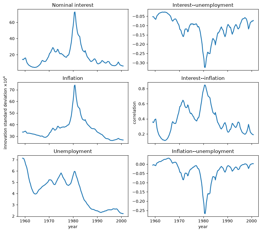
Fig. 93.4 Standard deviations and correlations implied by \(E(R_t\mid T)\)#
The interest-rate and inflation innovation standard deviations peak sharply around 1980, whereas unemployment innovation volatility declines more gradually toward the end of the sample.
All three innovation correlations also move most abruptly around 1980, so both the size and the joint composition of reduced-form shocks changed.
These movements give the changing-shocks, or bad-luck, explanation an important role, although the interest-rate innovation is not itself a structural monetary-policy shock.
The log determinant of the posterior mean covariance matrix summarizes the generalized one-step innovation variance [Whittle, 1953].
The following transformation summarizes generalized innovation variance.
sign, logdet_r = np.linalg.slogdet(r_mean)
assert np.all(sign > 0)
fig, ax = plt.subplots()
ax.plot(data['dates'], logdet_r, lw=2)
ax.set_xlabel('year')
ax.set_ylabel(r'$\log |E(R_t\mid T)|$')
plt.show()
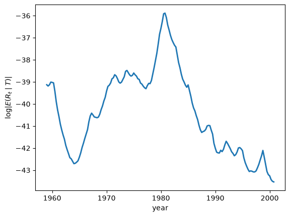
Fig. 93.5 Generalized innovation variance \(\log |E(R_t\mid T)|\)#
Because a less negative log determinant means greater joint innovation variance, the two-step rise to an exceptional 1981 peak and the long subsequent decline mark a large shock episode followed by the Great Moderation documented by Kim and Nelson [1999] and McConnell and Perez-Quiros [2000].
This is the clearest aggregate evidence for changing luck, but it cannot explain the coefficient-based changes in inflation dynamics examined next.
93.7.3. Core inflation and the natural rate#
To study the systematic dynamics, write the VAR at date \(t\) in companion form as
At date \(t\), the local mean \(m_t\) is the fixed point to which the companion-form VAR would converge if its coefficients remained fixed at their posterior means and future innovations were zero.
Here \(s_\pi\) and \(s_u\) select inflation and unemployment from \(m_t\), the factor four annualizes inflation, and the inverse-logit transformation returns unemployment to its observed rate.
These are date-specific steady states of frozen local systems rather than unconditional means of the globally drifting process.
Core inflation is the long-horizon inflation forecast implied by freezing the date-\(t\) coefficients, while the natural rate is the corresponding long-run unemployment anchor rather than a natural interest rate or a forecast of next quarter’s unemployment.
Freezing the current coefficients and projecting forward is exactly the anticipated-utility device used by the learning governments of Adaptive Learning and Escape Dynamics and Escaping Nash Inflation, who act as if their current beliefs will never be revised.
The following implementation annualizes core inflation and reverses the archive’s unemployment transformation.
def local_means(θ_path):
    """Compute local core inflation and the natural unemployment rate."""
    θ_path = np.asarray(θ_path, dtype=float)
    if θ_path.ndim == 1:
        θ_path = θ_path[:, None]
    core = np.empty(θ_path.shape[1])
    natural = np.empty(θ_path.shape[1])
    for t in range(θ_path.shape[1]):
        intercept, companion = companion_matrix(θ_path[:, t])
        mean = np.linalg.solve(np.eye(6) - companion, intercept)
        core[t] = 4 * mean[2]
        natural[t] = expit(100 * mean[1])
    return core, natural


core_inflation, natural_rate = local_means(θ_mean)
We plot the fourth-quarter observation from each year.
def annual_indices(dates, start=1960):
    """Return the final observation in each year from a start date."""
    year_values = np.floor(dates + 1e-8).astype(int)
    return np.array(
        [
            np.flatnonzero(year_values == year)[-1]
            for year in np.unique(year_values)
            if year >= start
        ]
    )


years = np.floor(data['dates'] + 1e-8).astype(int)
annual = annual_indices(data['dates'])

fig, ax = plt.subplots()
ax.plot(data['dates'][annual], 100 * core_inflation[annual], 'o-', lw=2,
        markersize=3, label='core inflation')
ax.plot(data['dates'][annual], 100 * natural_rate[annual], '+-', lw=2,
        markersize=5, label='natural rate')
ax.set_xlabel('year')
ax.set_ylabel('percent')
ax.legend()
plt.show()
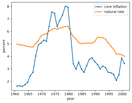
Fig. 93.6 Local means \(\bar\pi_t\) and \(\bar u_t\)#
core_summary = pd.Series(
    {
        'early-1960s mean core inflation (%)': (
            100 * core_inflation[(years >= 1960) & (years <= 1964)].mean()
        ),
        'peak core inflation (%)': 100 * core_inflation[annual].max(),
        '1985--2000 mean core inflation (%)': (
            100 * core_inflation[(years >= 1985) & (years <= 2000)].mean()
        ),
    },
    name='estimate',
)
core_summary.to_frame().round(2)
| estimate | |
|---|---|
| early-1960s mean core inflation (%) | 1.67 |
| peak core inflation (%) | 8.02 |
| 1985--2000 mean core inflation (%) | 3.09 |
Core inflation climbs from a low level in the early 1960s to a high peak near 1980 and then falls back, while the natural unemployment rate rises more smoothly from about 5 to 6.5 percent before returning toward 4 percent.
Because both lines are determined by the fitted coefficients rather than by realized shocks, their persistent shifts point to a changing systematic component.
The following calculation summarizes their comovement over the full posterior sample.
core_natural_correlation = np.corrcoef(core_inflation, natural_rate)[0, 1]

core_natural_correlation
np.float64(0.8375125177866256)
The strong positive quarterly correlation between \(\bar\pi_t\) and \(\bar u_t\) says that the model-implied long-run inflation and unemployment anchors share a broad cycle, not that current inflation and current unemployment must move together.
Because \((I-A_t)^{-1}\) amplifies small coefficient changes when the largest root is close to one, long-run means are intrinsically more sensitive than short-horizon forecasts.
93.7.4. Inflation persistence#
We now ask whether the systematic dynamics drifted on top of the moving volatilities.
The main summary is inflation persistence, measured by the normalized spectrum of inflation at frequency zero.
The spectral density of inflation at date \(t\) is
where \(\mathcal R_t\) embeds \(E(R_t\mid T)\) in the companion system.
Low-frequency power depends on both the autoregressive coefficients and the innovation covariance.
The next function evaluates inflation power at any frequency measured in cycles per quarter and also returns inflation variance at date \(t\).
def inflation_spectrum(θ, covariance, frequencies):
    """Compute inflation power and its variance-normalized counterpart."""
    _, companion = companion_matrix(θ)
    innovation = np.zeros((6, 6))
    innovation[:3, :3] = covariance
    selector = np.zeros(6)
    selector[2] = 1
    stationary = linalg.solve_discrete_lyapunov(companion, innovation)
    variance = float(selector @ stationary @ selector)
    power = np.empty(len(frequencies))
    for index, frequency in enumerate(frequencies):
        phase = np.exp(-2j * np.pi * frequency)
        transfer = np.linalg.solve(np.eye(6) - companion * phase, np.eye(6))
        power[index] = np.real(
            selector @ transfer @ innovation @ transfer.conj().T @ selector
        ) / (2 * np.pi)
    return power, power / variance
The normalized spectrum divides by inflation variance at date \(t\),
so \(g_{\pi\pi}(0,t)\) is an autocorrelation-based persistence measure.
The normalization removes a common scale factor from \(R_t\), but it can still depend on the relative variances and covariances in \(R_t\).
The first figure isolates frequency zero as a one-dimensional persistence summary.
zero_frequency = np.array([0.0])
inflation_persistence = np.array([
    inflation_spectrum(θ_mean[:, t], r_mean[t], zero_frequency)[1][0]
    for t in range(len(data['dates']))
])

fig, ax = plt.subplots()
ax.plot(
    data['dates'][annual],
    inflation_persistence[annual],
    'o-',
    lw=2,
    markersize=3,
)
ax.set_xlabel('year')
ax.set_ylabel(r'$g_{\pi\pi}(0,t)$')
plt.show()
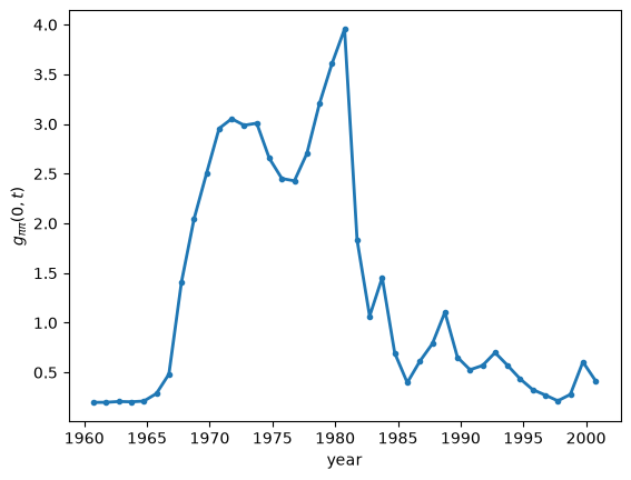
Fig. 93.7 Normalized zero-frequency spectrum \(g_{\pi\pi}(0,t)\)#
persistence_summary = pd.Series(
    {
        '1960--64 mean': inflation_persistence[
            (years >= 1960) & (years <= 1964)
        ].mean(),
        '1970--79 mean': inflation_persistence[
            (years >= 1970) & (years <= 1979)
        ].mean(),
        '1985--2000 mean': inflation_persistence[
            (years >= 1985) & (years <= 2000)
        ].mean(),
        'peak': inflation_persistence[annual].max(),
        'peak year': years[annual][np.argmax(inflation_persistence[annual])],
    },
    name='estimate',
)
persistence_summary.to_frame().round(3)
| estimate | |
|---|---|
| 1960--64 mean | 0.204 |
| 1970--79 mean | 2.865 |
| 1985--2000 mean | 0.537 |
| peak | 3.956 |
| peak year | 1980.000 |
Normalized zero-frequency power rises sharply from a low level in the early 1960s to a high peak around 1980 and then falls back below one for most of the remaining sample.
The post-1980 collapse cannot be explained by a proportional rescaling of all innovations, although the normalized statistic can still depend on the composition of \(R_t\).
For comparison, an \(AR(1)\) with coefficient \(\rho\) has normalized zero-frequency power \((1+\rho)/[2\pi(1-\rho)]\).
Values between 2 and 10 correspond to \(\rho\) between approximately \(0.85\) and \(0.97\).
The zero-frequency path omits the rest of the frequency distribution.
The following heatmaps show how raw and variance-normalized inflation power move over both time and frequency.
def inflation_spectrum_surface(θ_path, covariance_path, frequencies):
    """Evaluate the inflation spectrum at each date on a frequency grid."""
    raw = np.empty((len(frequencies), θ_path.shape[1]))
    normalized = np.empty_like(raw)
    for date in range(θ_path.shape[1]):
        raw[:, date], normalized[:, date] = inflation_spectrum(
            θ_path[:, date],
            covariance_path[date],
            frequencies,
        )
    return raw, normalized


spectrum_frequencies = np.linspace(0, 0.5, 41)
raw_spectrum, normalized_spectrum = inflation_spectrum_surface(
    θ_mean,
    r_mean,
    spectrum_frequencies,
)
spectrum_start = data['dates'] >= 1960
fig, axes = plt.subplots(1, 2, figsize=(9, 4), sharey=True)
surfaces = (
    (raw_spectrum, 'raw spectrum', 'log10 power'),
    (normalized_spectrum, 'normalized spectrum', 'log10 normalized power'),
)
for ax, (surface, title, color_label) in zip(axes, surfaces):
    image = ax.pcolormesh(
        data['dates'][spectrum_start],
        spectrum_frequencies,
        np.log10(surface[:, spectrum_start]),
        shading='auto',
    )
    ax.set_xlabel('year')
    ax.set_ylabel(f'{title}\ncycles per quarter')
    fig.colorbar(image, ax=ax, label=color_label)
plt.tight_layout()
plt.show()
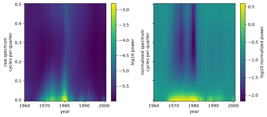
Fig. 93.8 Inflation spectra \(f_{\pi\pi}(\omega,t)\) and \(g_{\pi\pi}(\omega,t)\)#
The raw spectrum is brightest near frequency zero around 1980 because shocks and persistence are both elevated, while the normalized spectrum retains a broad low-frequency ridge through the 1970s that recedes after 1980.
The ridge that survives normalization shows that the Great Inflation was not only a high-volatility episode because inflation shocks were also propagated more persistently.
Point estimates do not reveal how strongly the data locate these paths.
We therefore compute the same annual features from every retained draw.
def posterior_feature_draws(result, indices):
    """Compute selected local means and persistence for retained draws."""
    n_draws = result['SD'].shape[2]
    shape = (len(indices), n_draws)
    core = np.empty(shape)
    natural = np.empty(shape)
    persistence = np.empty(shape)
    for draw in range(n_draws):
        core[:, draw], natural[:, draw] = local_means(
            result['SD'][:, indices, draw]
        )
        for row, date in enumerate(indices):
            covariance = innovation_covariance(
                result['HD'][date + 1, :, draw],
                result['CD'][:, draw],
            )
            persistence[row, draw] = inflation_spectrum(
                result['SD'][:, date, draw],
                covariance,
                zero_frequency,
            )[1][0]
    return {
        'core': 100 * core,
        'natural': 100 * natural,
        'persistence': persistence,
    }


historical_feature_draws = posterior_feature_draws(posterior, annual)
fig, axes = plt.subplots(3, 1, figsize=(9, 8), sharex=True)
feature_specs = (
    ('core', 'core inflation (%)'),
    ('natural', 'natural rate (%)'),
    ('persistence', r'$g_{\pi\pi}(0,t)$'),
)
for ax, (key, ylabel) in zip(axes, feature_specs):
    lower, median, upper = np.quantile(
        historical_feature_draws[key],
        (0.05, 0.5, 0.95),
        axis=1,
    )
    line, = ax.plot(data['dates'][annual], median, lw=2)
    ax.fill_between(
        data['dates'][annual],
        lower,
        upper,
        color=line.get_color(),
        alpha=0.2,
    )
    ax.set_ylabel(ylabel)
axes[-1].set_xlabel('year')
plt.tight_layout()
plt.show()
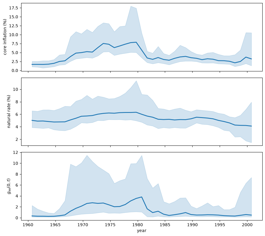
Fig. 93.9 Posterior medians and pointwise 90 percent intervals for \(\bar\pi_t\), \(\bar u_t\), and \(g_{\pi\pi}(0,t)\)#
The solid curves are posterior medians, and the shaded regions are pointwise 90 percent intervals rather than simultaneous bands for entire paths.
The median core-inflation and persistence paths preserve the rise and post-1980 fall, but their right-skewed bands widen markedly through the 1970s and around 1980.
The natural-rate median moves more smoothly, with broad uncertainty around 1980 and again at the sample endpoint, so the direction of the historical movement is clearer than its exact magnitude.
The following plot compares the timing of core inflation and persistence.
core_persistence_correlation = np.corrcoef(
    core_inflation, inflation_persistence
)[0, 1]

fig, ax = plt.subplots()
ax.plot(data['dates'][annual], 100 * core_inflation[annual], 'o-',
        lw=2, markersize=3, label='core inflation (%)')
ax.plot(data['dates'][annual], inflation_persistence[annual], 'x-',
        lw=2, markersize=4, label='normalized spectrum at zero')
ax.set_xlabel('year')
ax.legend()
plt.show()
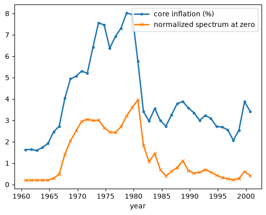
Fig. 93.10 \(\bar\pi_t\) and \(g_{\pi\pi}(0,t)\)#
Core inflation and normalized persistence rise together through the late 1960s and 1970s and collapse almost simultaneously after 1980, although core remains positive after persistence falls below one.
Their quarterly correlation of 0.909 summarizes common timing rather than a causal relationship because the two measures have different units and are nonlinear summaries of the same fitted coefficients.
Within the fitted TVP-VAR, the joint movement supports an important role for changing propagation as well as changing shock volatility.
A direct comparison with fixed coefficients requires fitting the restricted \(Q=0\) model.
The fall in persistence during the Volcker disinflation conflicts with escape-route models in which persistence grows along a transition from high to low inflation [Cho et al., 2002, Sargent, 1999].
That tension helped motivate later learning models in which policymakers became reluctant to disinflate during the 1970s and then changed course.
93.7.5. Monetary policy activism#
Cogley and Sargent summarize systematic policy with a forward-looking Taylor rule,
They define the activism coefficient as \(\mathcal A_t=\beta_1/(1-\beta_3)\) and call policy active when \(\mathcal A_t\geq 1\).
At each date, population two-stage least squares projections implied by the local VAR produce the policy-rule coefficients.
The benchmark horizons are \(h_\pi=4\) quarters and \(h_u=2\) quarters, reflecting conventional views about monetary-policy lags.
The following function projects the short rate on the model-implied inflation and unemployment forecasts using the stationary second moments of each local VAR.
def policy_rule_coefficients(θ, covariance, h_pi=4, h_u=2):
    """Return the local policy-rule coefficients."""
    _, companion = companion_matrix(θ)
    innovation = np.zeros((6, 6))
    innovation[:3, :3] = covariance
    stationary_covariance = linalg.solve_discrete_lyapunov(
        companion, innovation
    )
    selectors = np.eye(6)
    companion_power = np.eye(6)
    inflation_loading = np.zeros(6)
    unemployment_loading = np.zeros(6)
    for horizon in range(1, max(h_pi, h_u) + 1):
        companion_power = companion_power @ companion
        if horizon <= h_pi:
            inflation_loading += selectors[2] @ companion_power
        if horizon <= h_u:
            unemployment_loading += selectors[1] @ companion_power
    inflation_loading /= h_pi
    unemployment_loading /= h_u
    loadings = np.vstack(
        (inflation_loading, unemployment_loading, selectors[0])
    )
    regressor_covariance = loadings @ stationary_covariance @ loadings.T
    cross_covariance = (
        loadings @ stationary_covariance @ companion.T @ selectors[0]
    )
    return np.linalg.solve(regressor_covariance, cross_covariance)


policy_coefficients = np.array(
    [
        policy_rule_coefficients(θ_mean[:, t], r_mean[t])
        for t in range(len(data['dates']))
    ]
)
inflation_response = policy_coefficients[:, 0]
interest_persistence = policy_coefficients[:, 2]
policy_margin = np.where(
    np.abs(interest_persistence) < 1,
    inflation_response + interest_persistence - 1,
    np.nan,
)
For \(|\beta_3|<1\), the policy margin \(\mathcal{M}_t=\beta_{1t}+\beta_{3t}-1\) is nonnegative exactly when \(\mathcal A_t\geq1\) and avoids division by \(1-\beta_3\).
Because \(\beta_3\) multiplies the lagged interest rate, the long-run response sums \(\beta_1(1+\beta_3+\beta_3^2+\cdots)\) and exists only when \(|\beta_3|<1\).
The figures leave other dates blank because \(\mathcal A_t\) has no finite long-run interpretation there.
fig, ax = plt.subplots()
ax.plot(data['dates'], policy_margin, lw=2)
ax.axhline(0, color='0.45', lw=1)
ax.set_xlabel('year')
ax.set_ylabel(r'policy margin $\mathcal{M}_t$')
plt.show()
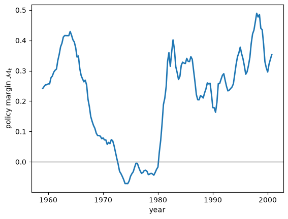
Fig. 93.11 Policy margin \(\mathcal{M}_t=\beta_{1t}+\beta_{3t}-1\)#
The policy margin falls below zero through much of the 1970s and then moves decisively above zero after the early 1980s.
This timing is consistent with a policy-regime contribution to the Great Inflation.
Blank intervals mark dates at which the policy margin is omitted by the rule above.
The following scatter plots use fourth-quarter observations.
displayed_annual = annual[np.isfinite(policy_margin[annual])]

fig, axes = plt.subplots(1, 2, figsize=(9, 4))
pairs = (
    (100 * core_inflation, 'core inflation (%)'),
    (inflation_persistence, 'normalized spectrum at zero'),
)
for ax, (feature, label) in zip(axes, pairs):
    ax.scatter(
        policy_margin[displayed_annual],
        feature[displayed_annual],
        s=18,
    )
    ax.axvline(0, color='0.45', lw=1)
    ax.set_xlabel(r'policy margin $\mathcal{M}_t$')
    ax.set_ylabel(label)
plt.tight_layout()
plt.show()
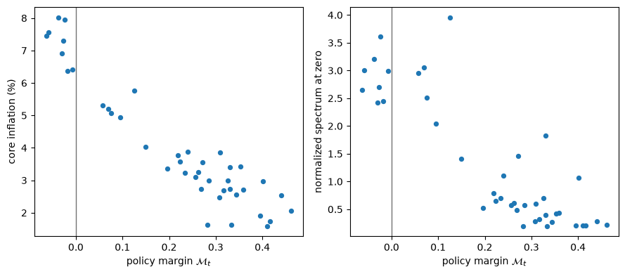
Fig. 93.12 \(\mathcal{M}_t\) versus \(\bar\pi_t\) and \(g_{\pi\pi}(0,t)\)#
High core-inflation and persistence observations cluster near or below the zero margin, whereas positive policy margins cluster at low values of both measures.
The displayed fourth-quarter observations establish a historical association rather than a causal policy effect.
The policy-rule coefficients are weakly identified at some dates, so a path based on posterior mean inputs understates uncertainty.
We therefore calculate activism from every retained draw in 1975, 1985, and 1995.
selected_years = (1975, 1985, 1995)
selected_dates = [np.flatnonzero(years == year)[-1] for year in selected_years]

activism_draws = {
    year: np.empty(posterior['SD'].shape[2]) for year in selected_years
}
stable_response_by_year = {
    year: np.empty(posterior['SD'].shape[2], dtype=bool)
    for year in selected_years
}
for draw in range(posterior['SD'].shape[2]):
    for year, date in zip(selected_years, selected_dates):
        covariance = innovation_covariance(
            posterior['HD'][date + 1, :, draw],
            posterior['CD'][:, draw],
        )
        rule = policy_rule_coefficients(
            posterior['SD'][:, date, draw], covariance
        )
        activism_draws[year][draw] = rule[0] / (1 - rule[2])
        stable_response_by_year[year][draw] = np.abs(rule[2]) < 1
These draws give posterior probabilities of active policy at each date and of a rise in activism after 1975, conditional on \(|\beta_3|<1\).
activism_events = (
    activism_draws[1975] > 1,
    activism_draws[1985] > 1,
    activism_draws[1995] > 1,
    activism_draws[1985] > activism_draws[1975],
    activism_draws[1995] > activism_draws[1975],
)
activism_conditions = (
    stable_response_by_year[1975],
    stable_response_by_year[1985],
    stable_response_by_year[1995],
    stable_response_by_year[1985] & stable_response_by_year[1975],
    stable_response_by_year[1995] & stable_response_by_year[1975],
)
assert all(condition.any() for condition in activism_conditions)
activism_probability_values = np.array(
    [
        event[condition].mean()
        for event, condition in zip(activism_events, activism_conditions)
    ]
)

activism_probability_index = (
    'P(A_1975 > 1)',
    'P(A_1985 > 1)',
    'P(A_1995 > 1)',
    'P(A_1985 > A_1975)',
    'P(A_1995 > A_1975)',
)
activism_probabilities = pd.DataFrame(
    {'conditional estimate': activism_probability_values},
    index=activism_probability_index,
)
stable_response_shares = pd.Series(
    {year: draws.mean() for year, draws in stable_response_by_year.items()},
    name='share with |beta_3| < 1',
)

display(activism_probabilities.round(3))
stable_response_shares.to_frame().round(3)
| conditional estimate | |
|---|---|
| P(A_1975 > 1) | 0.310 |
| P(A_1985 > 1) | 0.910 |
| P(A_1995 > 1) | 0.941 |
| P(A_1985 > A_1975) | 0.912 |
| P(A_1995 > A_1975) | 0.943 |
| share with |beta_3| < 1 | |
|---|---|
| 1975 | 1.000 |
| 1985 | 0.932 |
| 1995 | 0.980 |
The first three probabilities condition on \(|\beta_3|<1\) at that date, while the comparisons require this condition at both dates.
The central draw distributions expose the overlap and skewness behind the probability estimates.
stable_activism_draws = {
    year: activism_draws[year][stable_response_by_year[year]]
    for year in selected_years
}
pooled_activism = np.concatenate(tuple(stable_activism_draws.values()))
activism_limits = np.quantile(pooled_activism, (0.05, 0.95))
activism_bins = np.linspace(*activism_limits, 31)

fig, ax = plt.subplots()
for year in selected_years:
    central_draws = stable_activism_draws[year]
    central_draws = central_draws[
        (central_draws >= activism_limits[0])
        & (central_draws <= activism_limits[1])
    ]
    ax.hist(
        central_draws,
        bins=activism_bins,
        histtype='step',
        lw=2,
        label=str(year),
    )
ax.axvline(1, color='0.45', lw=1)
ax.set_xlabel('activism coefficient')
ax.set_ylabel('retained draws')
ax.legend()
plt.show()
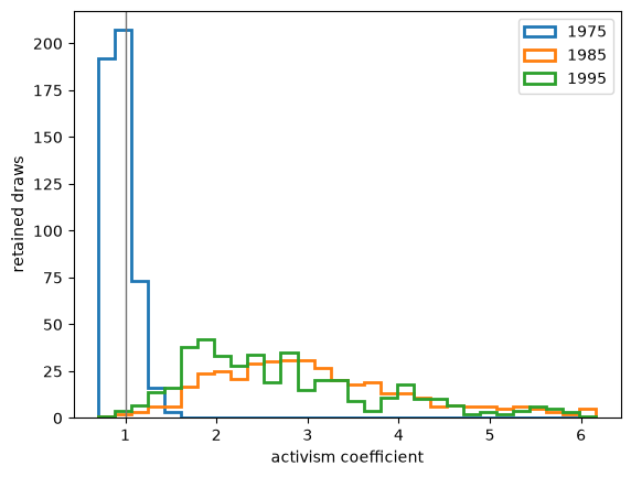
Fig. 93.13 Central posterior draws of \(\mathcal A_t\) conditional on \(|\beta_3|<1\) in 1975, 1985, and 1995#
The 1975 distribution is concentrated around or below one, while the 1985 and 1995 distributions shift substantially to the right but remain broad, skewed, and overlapping.
The posterior therefore favors a passive-to-active shift after 1975 but does not sharply distinguish 1985 from 1995.
The figure plots draws with \(|\beta_3|<1\) inside the pooled 5th and 95th percentiles, while the probability calculations use every such draw.
93.8. Another quarter-century of evidence#
The sample ends in 2000Q4, so it misses the financial crisis, the zero-interest-rate period, the pandemic, and the 2021–2022 inflation surge.
The question is whether these episodes alter the earlier evidence about drift, volatility, inflation persistence, and systematic policy.
93.8.1. The new observations#
To examine those observations, we append current data after 2000Q4 while leaving pre-2000Q4 sample unchanged.
This splice prevents revisions to pre-2001 CPI and unemployment data from being mistaken for information in the additional quarter-century.
We download seasonally adjusted CPI, seasonally adjusted unemployment, and the three-month Treasury-bill rate from FRED.
The transformations and within-quarter timing remain unchanged: CPI comes from the third month, unemployment is a three-month average, and the interest rate comes from the first month.
fred_url = (
    'https://fred.stlouisfed.org/graph/fredgraph.csv?'
    'id=CPIAUCSL%2CUNRATE%2CTB3MS'
)
fred_monthly = pd.read_csv(
    fred_url,
    parse_dates=['observation_date'],
).set_index('observation_date')
The BLS notes that the October 2025 unemployment observation was not collected during the federal government shutdown, leaving 2025Q4 without a complete three-month average.
The code below therefore ends the updated sample at the last quarter whose three monthly unemployment readings are all present, detected automatically rather than hard-coded; at the time of writing that quarter is 2025Q3.
def fred_quarterly_table(unemployment_monthly):
    """Construct transformed quarterly observations from current FRED data."""
    interest = fred_monthly.loc[
        fred_monthly.index.month.isin((1, 4, 7, 10)), 'TB3MS'
    ].copy()
    interest.index = interest.index.to_period('Q').start_time

    cpi = fred_monthly.loc[
        fred_monthly.index.month.isin((3, 6, 9, 12)), 'CPIAUCSL'
    ].copy()
    cpi.index = cpi.index.to_period('Q').start_time

    unemployment = unemployment_monthly.resample('QS').mean()
    quarterly = pd.concat(
        {
            'interest': interest,
            'unemployment': unemployment,
            'cpi': cpi,
        },
        axis=1,
    )
    quarterly['y3'] = np.log1p(quarterly['interest'] / 400)
    quarterly['ur'] = quarterly['unemployment'] / 100
    quarterly['dp'] = np.log(quarterly['cpi']).diff()
    quarterly['date'] = (
        quarterly.index.year + (quarterly.index.quarter - 1) / 4
    )
    columns = ['date', 'y3', 'ur', 'dp']
    return quarterly.loc[:, columns].dropna()


unemployment_monthly = fred_monthly['UNRATE']
unemployment_counts = unemployment_monthly.resample('QS').count()
latest_quarterly = fred_quarterly_table(unemployment_monthly)

# Extend the archived sample dynamically: append post-2000Q4 quarters only up
# to the first one missing any of its three monthly unemployment readings, so
# no endpoint is hard-coded.  An isolated missing month -- for example October
# 2025, which the federal shutdown left uncollected -- caps the sample at the
# preceding complete quarter, and a normally incomplete current quarter caps it
# at the last finished one.
quarterly_unfilled = latest_quarterly.loc['2001-01-01':]
month_counts = unemployment_counts.reindex(quarterly_unfilled.index)
incomplete_quarters = month_counts.index[month_counts < 3]
if len(incomplete_quarters):
    first_incomplete_quarter = incomplete_quarters[0]
    complete_extension = quarterly_unfilled.loc[
        quarterly_unfilled.index < first_incomplete_quarter
    ]
else:
    complete_extension = quarterly_unfilled

cs_sample = pd.read_csv(data_path)
overlap_date = pd.Timestamp('2000-10-01')
cs_sample_overlap = cs_sample.iloc[-1]
latest_overlap = latest_quarterly.loc[overlap_date]


def scaled_observation(row):
    """Return observable units for a transformed quarterly row."""
    return pd.Series(
        {
            'interest rate (annual %)': 400 * np.expm1(row['y3']),
            'unemployment (%)': 100 * row['ur'],
            'inflation (annual %)': 400 * row['dp'],
        }
    )


cs_sample_scaled = scaled_observation(cs_sample_overlap)
latest_scaled = scaled_observation(latest_overlap)
splice_audit = pd.DataFrame(
    {
        'Cogley-Sargent (2005) 2000Q4': cs_sample_scaled,
        'latest revised 2000Q4 data': latest_scaled,
        'current minus Cogley-Sargent (2005)': (
            latest_scaled - cs_sample_scaled
        ),
        'first appended 2001Q1': scaled_observation(
            complete_extension.iloc[0]
        ),
    }
)
extended_observations = pd.concat(
    (cs_sample, complete_extension.reset_index(drop=True)),
    ignore_index=True,
)


def quarter_label(timestamp):
    """Format a timestamp as year and quarter."""
    return str(timestamp.to_period('Q'))


display(splice_audit.round(3))
| Cogley-Sargent (2005) 2000Q4 | latest revised 2000Q4 data | current minus Cogley-Sargent (2005) | first appended 2001Q1 | |
|---|---|---|---|---|
| interest rate (annual %) | 6.253 | 6.110 | -0.143 | 5.150 |
| unemployment (%) | 3.967 | 3.900 | -0.067 | 4.233 |
| inflation (annual %) | 2.298 | 2.298 | -0.000 | 3.422 |
No missing value is filled or otherwise treated as observed.
The overlap table shows any break created by joining the archived data to the newly downloaded data.
The appended 2001Q1 inflation rate uses the latest revised CPI level for both 2000Q4 and 2001Q1, so one log difference never combines observations from two data releases.
fig, axes = plt.subplots(3, 1, figsize=(9, 7), sharex=True)
extended_plot = extended_observations[
    extended_observations['date'] >= 1959
]
updated_sample_end = complete_extension['date'].iloc[-1]
axes[0].plot(
    extended_plot['date'],
    400 * extended_plot['dp'],
    lw=2,
)
axes[0].set_ylabel('inflation (annual %)')
axes[1].plot(
    extended_plot['date'],
    100 * extended_plot['ur'],
    lw=2,
)
axes[1].set_ylabel('unemployment (%)')
axes[2].plot(
    extended_plot['date'],
    400 * np.expm1(extended_plot['y3']),
    lw=2,
)
axes[2].set_ylabel('interest (annual %)')
axes[2].set_xlabel('year')
for index, ax in enumerate(axes):
    cs_sample_label = 'Cogley-Sargent (2005)' if index == 0 else None
    sample_end_label = 'updated sample end' if index == 0 else None
    ax.axvline(
        2000.75,
        color='0.65',
        ls='--',
        lw=1,
        label=cs_sample_label,
    )
    ax.axvline(
        updated_sample_end,
        color='0.45',
        ls=':',
        lw=1,
        label=sample_end_label,
    )
axes[0].legend()
plt.tight_layout()
plt.show()
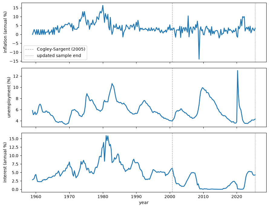
Fig. 93.14 Observed \(\pi_t\), \(u_t\), and \(i_t\), 1959Q1–2025Q3#
endpoint_observation = complete_extension.iloc[-1]
pd.Series(
    {
        'annualized quarterly inflation (%)': (
            400 * endpoint_observation['dp']
        ),
        'unemployment (%)': 100 * endpoint_observation['ur'],
        'three-month interest rate (%)': (
            400 * np.expm1(endpoint_observation['y3'])
        ),
    },
    name=quarter_label(complete_extension.index[-1]),
).to_frame().round(3)
| 2025Q3 | |
|---|---|
| annualized quarterly inflation (%) | 3.482 |
| unemployment (%) | 4.333 |
| three-month interest rate (%) | 4.250 |
The extension adds the financial-crisis contraction, a pandemic quarterly unemployment spike to 13.0 percent, and a short 2021–2022 inflation surge alongside two long stretches of near-zero interest rates.
Because inflation is annualized from quarterly changes, isolated movements look especially large in this panel, but the recent surge is still visibly much shorter than the sustained 1970s rise.
These observations provide a demanding test of whether the model assigns recent extremes to shock volatility or persistent dynamics, while the near-zero rate also weakens short-rate measures of policy after 2008.
We fit the stable TVP-VAR through 2025Q3, the last complete quarter, using the Treasury-bill measure above.
def append_extension(extension):
    """Append a transformed FRED extension to the Cogley-Sargent sample."""
    extension = extension.reset_index(drop=True)
    table = pd.concat((cs_sample, extension), ignore_index=True)
    assert table['date'].is_unique
    assert np.allclose(np.diff(table['date']), 0.25)
    return table


def fit_updated_model(table):
    """Calibrate and fit the stable drifting VAR to one table."""
    model_data = prepare_data(table)
    model_prior = calibrate_prior(model_data)
    result = run_sampler(
        model_data['y'],
        model_data['x'],
        model_prior,
        n_sweeps=5_000,
        burn=2_500,
        thin=5,
        seed=42,
        warmup=500,
        stable=True,
        progress_every=500,
    )
    validate_posterior_arrays(result, len(model_data['dates']))
    trace = np.trace(result['QD'], axis1=0, axis2=1)
    return {
        'data': model_data,
        'prior': model_prior,
        'posterior': result,
        'trace': trace,
    }


updated_fit = fit_updated_model(append_extension(complete_extension))

latest_data_table = latest_quarterly.loc[
    (latest_quarterly.index >= pd.Timestamp('1948-04-01'))
    & (latest_quarterly.index <= complete_extension.index[-1])
].reset_index(drop=True)
assert np.allclose(np.diff(latest_data_table['date']), 0.25)
latest_data_fit = fit_updated_model(latest_data_table)
500/5,000 sweeps; 907 slice contractions; 1.1 minutes
1,000/5,000 sweeps; 2,157 slice contractions; 2.2 minutes
1,500/5,000 sweeps; 3,239 slice contractions; 3.2 minutes
2,000/5,000 sweeps; 5,002 slice contractions; 4.4 minutes
2,500/5,000 sweeps; 6,186 slice contractions; 5.4 minutes
3,000/5,000 sweeps; 7,163 slice contractions; 6.5 minutes
3,500/5,000 sweeps; 7,943 slice contractions; 7.6 minutes
4,000/5,000 sweeps; 8,577 slice contractions; 8.6 minutes
4,500/5,000 sweeps; 9,404 slice contractions; 9.6 minutes
5,000/5,000 sweeps; 10,158 slice contractions; 10.7 minutes
500/5,000 sweeps; 862 slice contractions; 1.1 minutes
1,000/5,000 sweeps; 2,000 slice contractions; 2.1 minutes
1,500/5,000 sweeps; 3,099 slice contractions; 3.2 minutes
2,000/5,000 sweeps; 4,751 slice contractions; 4.3 minutes
2,500/5,000 sweeps; 6,298 slice contractions; 5.4 minutes
3,000/5,000 sweeps; 7,542 slice contractions; 6.5 minutes
3,500/5,000 sweeps; 8,617 slice contractions; 7.5 minutes
4,000/5,000 sweeps; 9,134 slice contractions; 8.6 minutes
4,500/5,000 sweeps; 9,568 slice contractions; 9.6 minutes
5,000/5,000 sweeps; 10,764 slice contractions; 10.7 minutes
93.8.2. Did coefficient drift continue?#
def updated_drift_summary(fit):
    """Summarize the updated coefficient-drift distribution."""
    trace = fit['trace']
    q_mean = fit['posterior']['QD'].mean(axis=2)
    eigenvalues = np.linalg.eigvalsh(q_mean)[::-1]
    return {
        'posterior mean tr(Q)': trace.mean(),
        'share in first three eigen-directions': (
            eigenvalues[:3].sum() / eigenvalues.sum()
        ),
    }


updated_label = quarter_label(complete_extension.index[-1])
updated_summary = pd.DataFrame(
    {
        'Cogley-Sargent (2005) + extension': (
            updated_drift_summary(updated_fit)
        ),
        'latest revised data for full sample': updated_drift_summary(
            latest_data_fit
        ),
    }
)
updated_summary.round(3)
| Cogley-Sargent (2005) + extension | latest revised data for full sample | |
|---|---|---|
| posterior mean tr(Q) | 0.073 | 0.034 |
| share in first three eigen-directions | 0.976 | 0.955 |
The drift-rate distributions and coefficient paths provide the same views used for the Cogley and Sargent [2005] sample.
The dashed vertical line in updated time-series figures marks the Cogley and Sargent [2005] sample’s 2000Q4 endpoint, but each updated path comes from a full re-estimation rather than from attaching new points to an unchanged historical estimate.
fig, ax = plt.subplots()
ax.hist(updated_fit['trace'], bins=30, histtype='step', lw=2)
ax.axvline(
    np.trace(updated_fit['prior']['q_center']),
    color='C1',
    lw=2,
    label=r'prior $\mathrm{tr}(\bar Q)$',
)
ax.set_xlabel(r'$\mathrm{tr}(Q)$')
ax.set_ylabel('frequency')
ax.legend()
plt.show()
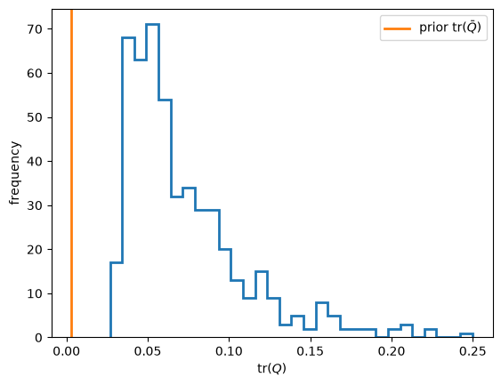
Fig. 93.15 Posterior \(\operatorname{tr}(Q)\) and prior \(\operatorname{tr}(\bar Q)\) through 2025Q3#
In both data constructions, the full-sample posterior drift rate remains above its conservative prior calibration.
Within the TVP-VAR this indicates non-negligible full-sample drift, but it is not a formal comparison of \(Q=0\) with \(Q>0\).
Its magnitude depends on whether the historical observations come from the archived dataset or the latest revisions.
Because \(Q\) is a single variance parameter for the full 1959–2025 path, this histogram does not by itself show that drift accelerated after 2000.
fig, axes = plt.subplots(1, 3, figsize=(10, 4), sharex=True)
updated_dates = updated_fit['data']['dates']
updated_coefficients = updated_fit['posterior']['SD'].mean(axis=2)
coefficient_lines = plot_equation_coefficients(
    axes,
    updated_dates,
    updated_coefficients,
)
for ax in axes:
    ax.axvline(2000.75, color='0.65', ls='--', lw=1)
fig.legend(
    coefficient_lines,
    coefficient_labels,
    loc='lower center',
    ncol=4,
)
plt.tight_layout(rect=(0, 0.17, 1, 1))
plt.show()
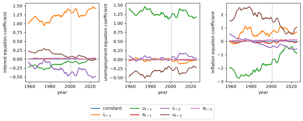
Fig. 93.16 Posterior mean VAR coefficients \(E(\theta_t\mid T)\) through 2025Q3#
Several coefficient paths continue moving gradually after 2000, with the largest changes again concentrated in the inflation equation rather than appearing as abrupt financial-crisis or pandemic breaks.
The opposing movements of some paired lag coefficients also show why their combined dynamic implications are more informative than any single line.
The first three eigen-directions account for the large majority of the posterior mean drift variance, so the estimated movement remains low dimensional.
The stability restriction now applies to a longer path, which makes the posterior drift rate a property of the full 1959–2025 sample.
93.8.3. Volatility after the Great Moderation#
We next separate changes in the sizes and correlations of innovations from changes in the VAR dynamics.
def model_features(fit):
    """Compute features at posterior mean parameters."""
    result = fit['posterior']
    θ = result['SD'].mean(axis=2)
    mean_root_modulus = np.max(
        np.abs(companion_roots(θ)), axis=1
    )
    if not np.all(mean_root_modulus < 1):
        raise ValueError('mean coefficient path is unstable')
    covariance = mean_innovation_covariance(result['HD'], result['CD'])
    core, natural = local_means(θ)
    persistence = np.array([
        inflation_spectrum(
            θ[:, t], covariance[t], zero_frequency
        )[1][0]
        for t in range(len(fit['data']['dates']))
    ])
    sign, logdet = np.linalg.slogdet(covariance)
    assert np.all(sign > 0)
    policy_coefficients = np.array(
        [
            policy_rule_coefficients(θ[:, t], covariance[t])
            for t in range(len(fit['data']['dates']))
        ]
    )
    inflation_response = policy_coefficients[:, 0]
    interest_persistence = policy_coefficients[:, 2]
    policy_margin = np.where(
        np.abs(interest_persistence) < 1,
        inflation_response + interest_persistence - 1,
        np.nan,
    )
    return {
        'θ': θ,
        'maximum_companion_root': mean_root_modulus.max(),
        'covariance': covariance,
        'core': core,
        'natural': natural,
        'persistence': persistence,
        'logdet': logdet,
        'policy_margin': policy_margin,
    }


updated_features = model_features(updated_fit)
latest_data_features = model_features(latest_data_fit)

pd.Series(
    {
        'Cogley-Sargent (2005) + extension': (
            updated_features['maximum_companion_root']
        ),
        'latest revised data for full sample': (
            latest_data_features['maximum_companion_root']
        ),
    },
    name='maximum companion-root modulus of mean path',
).to_frame().round(4)
| maximum companion-root modulus of mean path | |
|---|---|
| Cogley-Sargent (2005) + extension | 0.9569 |
| latest revised data for full sample | 0.9613 |
fig, axes = plt.subplots(3, 2, figsize=(9, 8), sharex=True)
dates = updated_fit['data']['dates']
covariance = updated_features['covariance']
for row, (index, _) in enumerate(variances):
    axes[row, 0].plot(
        dates,
        10000 * np.sqrt(covariance[:, index, index]),
        lw=2,
    )
for row, (left, right, _) in enumerate(correlations):
    scale = np.sqrt(
        covariance[:, left, left] * covariance[:, right, right]
    )
    axes[row, 1].plot(
        dates,
        covariance[:, left, right] / scale,
        lw=2,
    )
for row, (_, label) in enumerate(variances):
    axes[row, 0].set_title(label)
for row, (_, _, label) in enumerate(correlations):
    axes[row, 1].set_title(label)
for ax in axes.flat:
    ax.axvline(2000.75, color='0.65', ls='--', lw=1)
axes[1, 0].set_ylabel(
    r'innovation standard deviation $\times 10^4$'
)
axes[1, 1].set_ylabel('correlation')
axes[-1, 0].set_xlabel('year')
axes[-1, 1].set_xlabel('year')
plt.tight_layout()
plt.show()
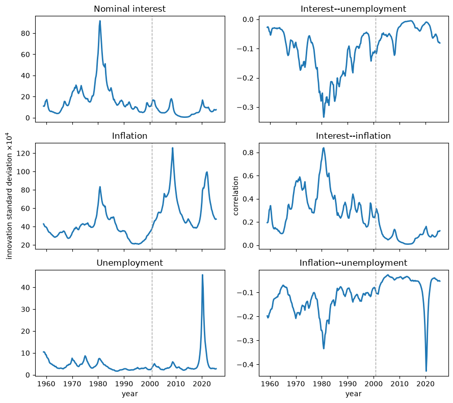
Fig. 93.17 Standard deviations and correlations implied by \(E(R_t\mid T)\) through 2025Q3#
The Volcker transition still dominates interest-rate innovation volatility, the financial crisis produces the largest inflation-volatility spike, and the pandemic uniquely dominates unemployment volatility.
The pandemic also drives a sharp fall in the inflation–unemployment correlation, so recent episodes changed the mix of reduced-form shocks as well as their size.
This is direct evidence for a bad-luck component, although reduced-form innovations do not establish that the underlying disturbances were structurally exogenous.
fig, ax = plt.subplots()
ax.plot(
    updated_fit['data']['dates'],
    updated_features['logdet'],
    lw=2,
)
ax.axvline(2000.75, color='0.65', ls='--', lw=1)
ax.set_xlabel('year')
ax.set_ylabel(r'$\log |E(R_t\mid T)|$')
plt.show()
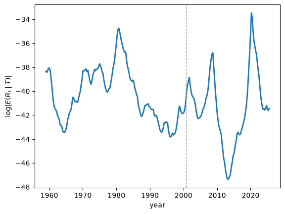
Fig. 93.18 \(\log |E(R_t\mid T)|\) through 2025Q3#
Joint innovation variance rises during the financial crisis, reaches a deep Great Moderation trough in the 2010s, and then jumps in 2020 above even its 1981 peak before falling rapidly.
def decimal_quarter_label(value):
    """Format a decimal quarterly date."""
    year = int(np.floor(value + 1e-8))
    quarter = int(round(4 * (value - year))) + 1
    return f'{year}Q{quarter}'


def volatility_summary(fit, features):
    """Summarize innovation-volatility peaks and endpoints."""
    dates = fit['data']['dates']
    standard_deviation = 10000 * np.sqrt(
        np.diagonal(features['covariance'], axis1=1, axis2=2)
    )
    names = ('interest', 'unemployment', 'inflation')
    return pd.DataFrame(
        {
            'peak quarter': [
                decimal_quarter_label(
                    dates[np.argmax(standard_deviation[:, index])]
                )
                for index in range(n_variables)
            ],
        },
        index=names,
    )


updated_volatility = volatility_summary(updated_fit, updated_features)
updated_volatility
| peak quarter | |
|---|---|
| interest | 1980Q4 |
| unemployment | 2020Q2 |
| inflation | 2008Q4 |
All three innovation standard deviations are well below their peaks at the 2025Q3 endpoint, which supports a large but transient pandemic-shock interpretation inside this model.
93.8.4. Core inflation and the natural rate after 2000#
The same local-mean calculation distinguishes temporary inflation from a shift in the model’s long-horizon forecast.
updated_dates = updated_fit['data']['dates']
updated_annual = annual_indices(updated_dates)
fig, ax = plt.subplots()
ax.plot(
    updated_dates[updated_annual],
    100 * updated_features['core'][updated_annual],
    'o-',
    lw=2,
    markersize=3,
    label='core inflation',
)
ax.plot(
    updated_dates[updated_annual],
    100 * updated_features['natural'][updated_annual],
    '+-',
    lw=2,
    markersize=5,
    label='natural rate',
)
ax.axvline(2000.75, color='0.65', ls='--', lw=1)
ax.set_xlabel('year')
ax.set_ylabel('percent')
ax.legend()
plt.show()
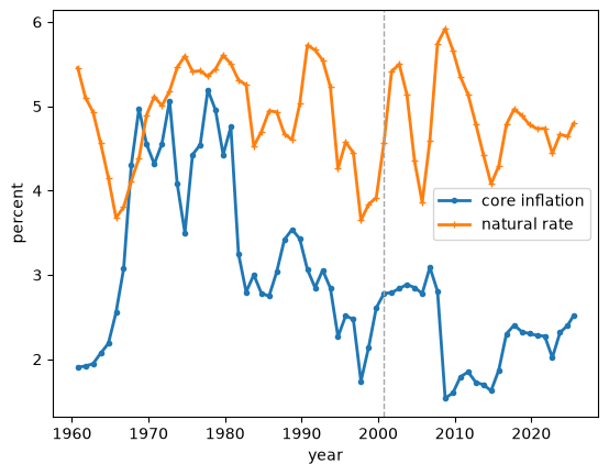
Fig. 93.19 Local means \(\bar\pi_t\) and \(\bar u_t\) through 2025Q3#
The 1970s core-inflation peak is lower here than in the Cogley and Sargent [2005] figure because later observations revise the smoothed history, so values on both sides of the dashed line belong to one updated fit.
After 2000 the core rate stays mostly between about 2 and 3 percent and rises only modestly after 2020, even though observed inflation moves much more sharply.
The natural-rate line is the model’s locally implied long-run unemployment anchor, which is why quarterly unemployment can jump to 13.0 percent in 2020 while this line remains near 5 percent.
The monthly peak was 14.8 percent.
The final annual point represents 2025Q3 because the sample ends before the fourth quarter.
def endpoint_features(features):
    """Return economically scaled endpoint features."""
    return pd.Series(
        {
            'core inflation (%)': 100 * features['core'][-1],
            'natural rate (%)': 100 * features['natural'][-1],
            'normalized persistence': features['persistence'][-1],
            'log generalized innovation variance': features['logdet'][-1],
        }
    )


updated_endpoints = endpoint_features(updated_features).to_frame(
    name=updated_label
).T
latest_data_endpoints = endpoint_features(
    latest_data_features
).to_frame(name=updated_label).T
data_revision_sensitivity = pd.concat(
    {
        'Cogley-Sargent (2005) + extension': updated_endpoints,
        'latest revised data for full sample': latest_data_endpoints,
    }
)
data_revision_sensitivity.round(3)
| core inflation (%) | natural rate (%) | normalized persistence | log generalized innovation variance | ||
|---|---|---|---|---|---|
| Cogley-Sargent (2005) + extension | 2025Q3 | 2.514 | 4.794 | 0.304 | -41.454 |
| latest revised data for full sample | 2025Q3 | 2.387 | 4.539 | 0.250 | -41.075 |
The endpoint core-inflation, natural-rate, and persistence summaries are similar across the two data constructions.
The draw-wise annual paths show how uncertainty evolves inside the updated fit.
updated_feature_draws = posterior_feature_draws(
    updated_fit['posterior'],
    updated_annual,
)
fig, axes = plt.subplots(3, 1, figsize=(9, 8), sharex=True)
for ax, (key, ylabel) in zip(axes, feature_specs):
    lower, median, upper = np.quantile(
        updated_feature_draws[key],
        (0.05, 0.5, 0.95),
        axis=1,
    )
    line, = ax.plot(updated_dates[updated_annual], median, lw=2)
    ax.fill_between(
        updated_dates[updated_annual],
        lower,
        upper,
        color=line.get_color(),
        alpha=0.2,
    )
    ax.axvline(2000.75, color='0.65', ls='--', lw=1)
    ax.set_ylabel(ylabel)
axes[-1].set_xlabel('year')
plt.tight_layout()
plt.show()
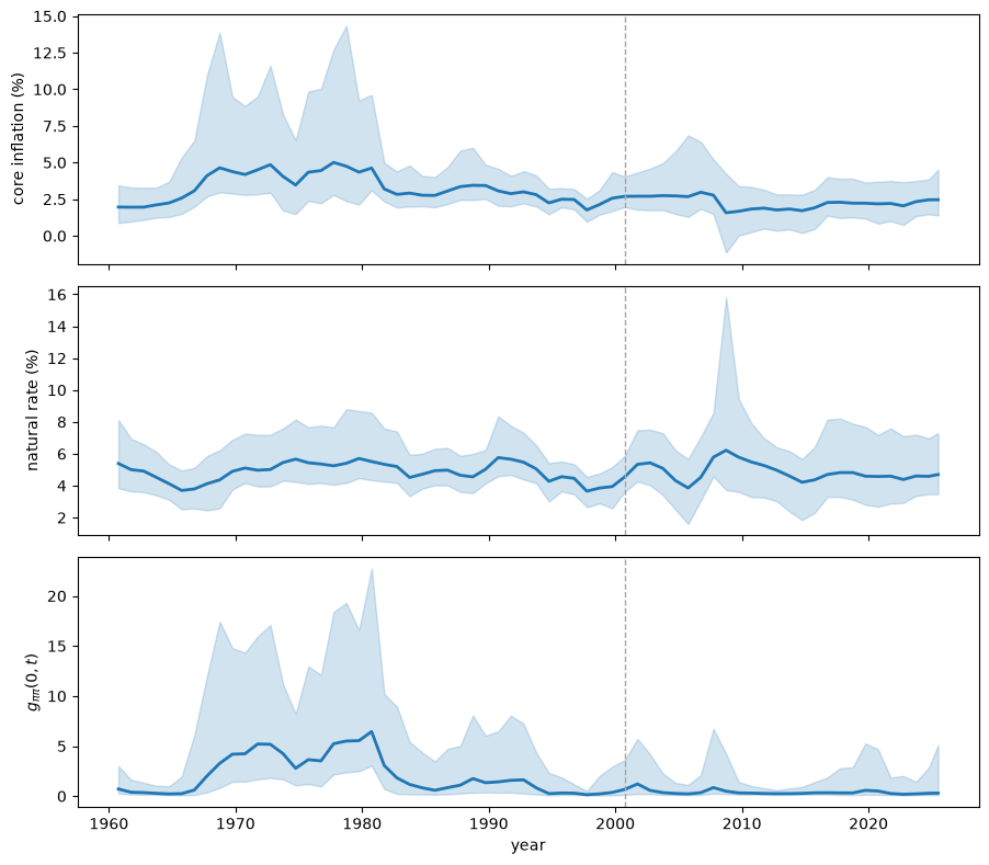
Fig. 93.20 Posterior medians and pointwise 90 percent intervals for \(\bar\pi_t\), \(\bar u_t\), and \(g_{\pi\pi}(0,t)\) through 2025Q3#
The solid lines are posterior medians, and the shaded regions are pointwise 90 percent intervals rather than simultaneous whole-path bands.
After 2000 the core-inflation median is comparatively flat and the persistence median remains low, whereas the natural-rate band is broad and widens again at the endpoint.
The endpoint rows summarize uncertainty in the three nonlinear features.
def endpoint_feature_intervals(draws):
    """Summarize draw-wise uncertainty in endpoint model features."""
    labels = {
        'core': 'core inflation (%)',
        'natural': 'natural rate (%)',
        'persistence': 'normalized persistence',
    }
    rows = {}
    for key, label in labels.items():
        values = draws[key][-1]
        rows[label] = {
            'median': np.median(values),
            '5th percentile': np.quantile(values, 0.05),
            '95th percentile': np.quantile(values, 0.95),
        }
    return pd.DataFrame.from_dict(rows, orient='index')


updated_endpoint_intervals = endpoint_feature_intervals(
    updated_feature_draws
)
updated_endpoint_intervals.round(3)
| median | 5th percentile | 95th percentile | |
|---|---|---|---|
| core inflation (%) | 2.463 | 1.383 | 4.529 |
| natural rate (%) | 4.698 | 3.470 | 7.302 |
| normalized persistence | 0.301 | 0.107 | 5.102 |
At 2025Q3 both the core-inflation and natural-rate medians remain historically moderate, as the table above shows.
Their intervals remain broad, and normalized persistence retains a substantial upper tail, so the classification of recent inflation as temporary is not certain.
93.8.5. Did inflation become persistent again?#
Here persistence means propagation of an inflation innovation into future inflation, rather than the number of quarters in which observed inflation remains high.
The normalized spectrum reduces sensitivity to a common change in shock scale, although it still depends on the relative variances and covariances in \(R_t\).
fig, ax = plt.subplots()
ax.plot(
    updated_dates[updated_annual],
    updated_features['persistence'][updated_annual],
    'o-',
    lw=2,
    markersize=3,
)
ax.axvline(2000.75, color='0.65', ls='--', lw=1)
ax.set_xlabel('year')
ax.set_ylabel(r'$g_{\pi\pi}(0,t)$')
plt.show()
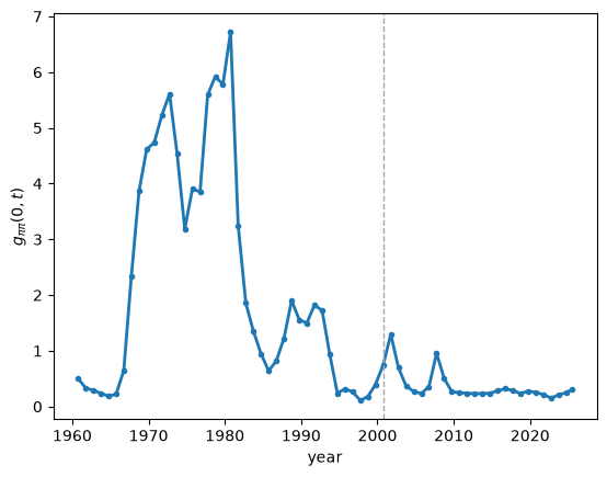
Fig. 93.21 \(g_{\pi\pi}(0,t)\) through 2025Q3#
The estimated \(g_{\pi\pi}(0,t)\) path recreates the rise to a 1980 peak and the subsequent collapse, but it stays near 0.2–0.5 after 2000 and rises only slightly after 2020.
A sequence of large reduced-form innovations can keep observed inflation high for several quarters without generating the strong propagation estimated for the 1970s.
fig, axes = plt.subplots(
    2,
    1,
    figsize=(9, 6),
    sharex=True,
)
axes[0].plot(
    updated_dates[updated_annual],
    100 * updated_features['core'][updated_annual],
    'o-',
    lw=2,
    markersize=3,
)
axes[1].plot(
    updated_dates[updated_annual],
    updated_features['persistence'][updated_annual],
    'x-',
    lw=2,
    markersize=4,
)
for ax in axes:
    ax.axvline(2000.75, color='0.65', ls='--', lw=1)
axes[0].set_ylabel('core inflation (%)')
axes[1].set_ylabel('normalized spectrum at zero')
axes[1].set_xlabel('year')
plt.tight_layout()
plt.show()
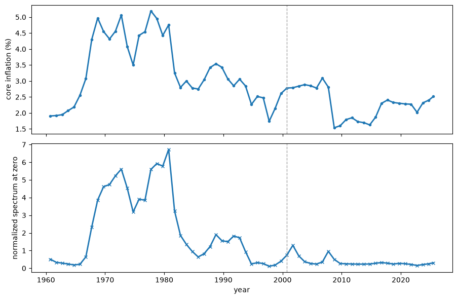
Fig. 93.22 \(\bar\pi_t\) and \(g_{\pi\pi}(0,t)\) through 2025Q3#
Core inflation recovers from its mid-2010s low toward its earlier level, while persistence remains in its low post-1980 range instead of rising with it.
This divergence separates a modest rise in the model’s long-run inflation rate from a return to 1970s-style propagation.
The full spectrum shows where the difference comes from.
updated_raw_spectrum, updated_normalized_spectrum = (
    inflation_spectrum_surface(
        updated_features['θ'],
        updated_features['covariance'],
        spectrum_frequencies,
    )
)
fig, axes = plt.subplots(
    1,
    2,
    figsize=(9, 4),
    sharey=True,
    constrained_layout=True,
)
updated_surfaces = (
    (updated_raw_spectrum, 'raw spectrum', 'log10 power'),
    (
        updated_normalized_spectrum,
        'normalized spectrum',
        'log10 normalized power',
    ),
)
for ax, (surface, title, color_label) in zip(axes, updated_surfaces):
    image = ax.pcolormesh(
        updated_dates,
        spectrum_frequencies,
        np.log10(surface),
        shading='auto',
    )
    ax.axvline(2000.75, color='0.85', ls='--', lw=1)
    ax.set_xlabel('year')
    ax.set_ylabel(f'{title}\ncycles per quarter')
    fig.colorbar(image, ax=ax, label=color_label)
plt.show()
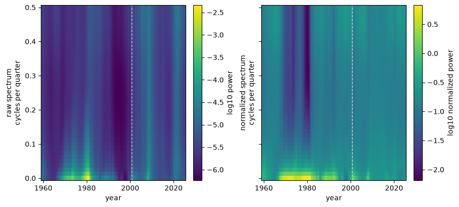
Fig. 93.23 \(f_{\pi\pi}(\omega,t)\) and \(g_{\pi\pi}(\omega,t)\) through 2025Q3#
The financial crisis and pandemic appear as bright, broad bands in \(f_{\pi\pi}(\omega,t)\) because reduced-form innovation variance increased.
The normalized spectrum \(g_{\pi\pi}(\omega,t)\) lacks a post-2000 low-frequency ridge comparable to the 1970s.
Together, the panels weigh against a return to 1970s-style persistence without making the normalized statistic independent of \(R_t\).
def episode_summary(fit, features):
    """Average selected features over economically distinct episodes."""
    years = np.floor(fit['data']['dates'] + 1e-8).astype(int)
    periods = {
        '1970--1979': (years >= 1970) & (years <= 1979),
        '1985--2000': (years >= 1985) & (years <= 2000),
        '2001--2019': (years >= 2001) & (years <= 2019),
        '2020--2022': (years >= 2020) & (years <= 2022),
        '2023--2025Q3': years >= 2023,
    }
    rows = {}
    for label, mask in periods.items():
        rows[label] = {
            'core inflation (%)': 100 * features['core'][mask].mean(),
            'normalized persistence': features['persistence'][mask].mean(),
            'log generalized innovation variance': (
                features['logdet'][mask].mean()
            ),
        }
    return pd.DataFrame.from_dict(rows, orient='index')


updated_episodes = episode_summary(updated_fit, updated_features)
updated_episodes.round(3)
| core inflation (%) | normalized persistence | log generalized innovation variance | |
|---|---|---|---|
| 1970--1979 | 4.518 | 4.756 | -38.614 |
| 1985--2000 | 2.786 | 0.914 | -42.006 |
| 2001--2019 | 2.293 | 0.414 | -42.099 |
| 2020--2022 | 2.226 | 0.229 | -36.432 |
| 2023--2025Q3 | 2.343 | 0.228 | -41.306 |
The episode averages contrast the high volatility of 2020–2022 with the lower normalized persistence of the post-2000 decades.
93.8.6. Can recent policy activism be measured?#
When \(|\beta_3|<1\), the policy margin gives the same active-policy classification after 2000 without division by \(1-\beta_3\).
In the following figures, the gray line marks the active-policy threshold \(\mathcal{M}_t=0\).
fig, ax = plt.subplots()
updated_policy_margin = updated_features['policy_margin']
ax.plot(updated_dates, updated_policy_margin, lw=2)
ax.axhline(0, color='0.45', lw=1)
ax.axvline(2000.75, color='0.65', ls='--', lw=1)
ax.set_xlabel('year')
ax.set_ylabel(r'policy margin $\mathcal{M}_t$')
plt.show()
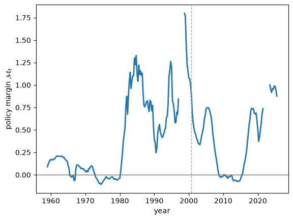
Fig. 93.24 Policy margin \(\mathcal{M}_t\) through 2025Q3#
Among the displayed post-2000 dates, the margin is mostly positive and moves toward zero in the mid-2010s and around 2020.
Blank intervals omit dates for which the fitted interest-rate response does not settle down.
fig, axes = plt.subplots(1, 2, figsize=(9, 4))
recent_annual = annual_indices(updated_dates, start=2001)
displayed_recent = recent_annual[
    np.isfinite(updated_policy_margin[recent_annual])
]
axes[0].scatter(
    updated_policy_margin[displayed_recent],
    100 * updated_features['core'][displayed_recent],
    s=18,
)
axes[1].scatter(
    updated_policy_margin[displayed_recent],
    updated_features['persistence'][displayed_recent],
    s=18,
)
for ax in axes:
    ax.axvline(0, color='0.45', lw=1)
    ax.set_xlabel(r'policy margin $\mathcal{M}_t$')
axes[0].set_ylabel('core inflation (%)')
axes[1].set_ylabel('normalized spectrum at zero')
plt.tight_layout()
plt.show()
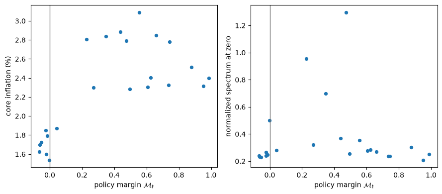
Fig. 93.25 Post-2000 \(\mathcal{M}_t\) versus \(\bar\pi_t\) and \(g_{\pi\pi}(0,t)\)#
The remaining post-2000 observations do not establish a stable causal relation between the policy margin, core inflation, and persistence.
We also examine the central draw distribution at the 2025Q3 endpoint.
def endpoint_policy_margin_draws(fit):
    """Return endpoint margins and stability indicators."""
    result = fit['posterior']
    margins = np.empty(result['SD'].shape[2])
    stable_response = np.empty(result['SD'].shape[2], dtype=bool)
    for draw in range(len(margins)):
        covariance = innovation_covariance(
            result['HD'][-1, :, draw],
            result['CD'][:, draw],
        )
        rule = policy_rule_coefficients(
            result['SD'][:, -1, draw], covariance
        )
        margins[draw] = rule[0] + rule[2] - 1
        stable_response[draw] = np.abs(rule[2]) < 1
    return margins, stable_response


updated_margin_draws, stable_response_draws = (
    endpoint_policy_margin_draws(updated_fit)
)
assert np.any(stable_response_draws)
stable_margin_draws = updated_margin_draws[stable_response_draws]
updated_margin_summary = pd.Series(
    {
        'median M': np.median(stable_margin_draws),
        '5th percentile of M': np.quantile(stable_margin_draws, 0.05),
        '95th percentile of M': np.quantile(stable_margin_draws, 0.95),
        'P(M >= 0 | |beta_3| < 1)': np.mean(stable_margin_draws >= 0),
        'share with |beta_3| < 1': stable_response_draws.mean(),
    },
    name=updated_label,
).to_frame().T
updated_margin_summary.round(3)
| median M | 5th percentile of M | 95th percentile of M | P(M >= 0 | |beta_3| < 1) | share with |beta_3| < 1 | |
|---|---|---|---|---|---|
| 2025Q3 | 0.383 | -0.643 | 1.121 | 0.904 | 0.732 |
updated_margin_limits = np.quantile(
    stable_margin_draws,
    (0.05, 0.95),
)
updated_margin_bins = np.linspace(*updated_margin_limits, 31)

fig, ax = plt.subplots()
central_draws = stable_margin_draws[
    (stable_margin_draws >= updated_margin_limits[0])
    & (stable_margin_draws <= updated_margin_limits[1])
]
ax.hist(
    central_draws,
    bins=updated_margin_bins,
    histtype='step',
    lw=2,
)
ax.axvline(0, color='0.45', lw=1)
ax.set_xlabel(r'policy margin $\mathcal{M}_t$')
ax.set_ylabel('draw count')
plt.show()
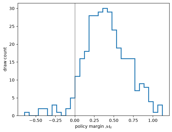
Fig. 93.26 Central 90 percent of posterior draws for \(\mathcal{M}_t\) conditional on \(|\beta_3|<1\) at 2025Q3#
The table reports the share of draws with a stable interest-rate response and the active-policy probability among those draws.
An interval spanning zero indicates that the endpoint classification remains uncertain.
The plot displays only draws between the 5th and 95th percentiles, and the zero lower bound and unconventional policy further weaken the interpretation of this short-rate projection after 2008.
93.8.7. What the additional observations change#
The extra quarter-century adds a dramatic volatility episode without a post-2000 low-frequency ridge comparable to the 1970s.
The pandemic is the dominant aggregate uncertainty episode, but the recent inflation surge does not reproduce the 1970s low-frequency persistence ridge.
Within the updated TVP-VAR, the full-sample drift-rate posterior remains above its conservative prior calibration; a fixed-coefficient comparison would require a separate \(Q=0\) model.
The 2025Q3 natural-rate and policy-margin estimates remain imprecise, especially because not every posterior draw satisfies \(|\beta_3|<1\).
93.9. Bad policy or bad luck? A verdict#
The Bayesian VAR delivers a nuanced answer to the question that opened this lecture.
Volatilities drifted: the size of the shocks changed enormously, with a Volcker-era spike and a subsequent Great Moderation, so the bad-luck story captures something real.
The fitted TVP-VAR attributes variation to coefficients too: inflation persistence and core inflation rose through the 1970s and fell in the 1980s, although a formal fixed-versus-drifting comparison requires a separate \(Q=0\) model.
The new observations do not overturn that distinction: the pandemic produces an extreme volatility episode, while the recent inflation surge does not recreate the persistence of the 1970s.
The reduced-form VAR cannot by itself prove that changes in Federal Reserve beliefs caused the coefficient drift, because private behavior and other omitted mechanisms can also change reduced-form dynamics.
There is one more twist, and it loops us back to the theory of this section.
The escape-route models of Adaptive Learning and Escape Dynamics and Escaping Nash Inflation predict that inflation persistence should grow along a disinflation as a learning government becomes reluctant to abandon a high-inflation self-confirming equilibrium.
The data show the opposite because persistence fell as inflation came down after 1980.
It helped motivate later learning models, including Cogley and Sargent [2005] and Primiceri [2006], in which policymakers’ reluctance to disinflate in the 1970s and their eventual conversion generate persistence that first rises and then falls.
The friendly debate with Sims, Zha, Bernanke, and Mihov thus did more than adjudicate a historical question.
It sharpened the theoretical models of learning and drift that run through this section, from the self-confirming equilibria of the Conquest book to the drifting Fed beliefs used to interpret later inflation.
93.10. Exercises#
Exercise 93.1
For an \(AR(1)\) process, normalized zero-frequency power is
Compute \(g(0)\) for \(\rho=0\), \(0.85\), and \(0.97\), and use the persistence path above to interpret how inflation dynamics changed around 1980.
Solution
ρ = np.array([0.0, 0.85, 0.97])
g0 = (1 + ρ) / (2 * np.pi * (1 - ρ))
pd.Series(g0, index=ρ, name='normalized power at zero').to_frame()
| normalized power at zero | |
|---|---|
| 0.00 | 0.159155 |
| 0.85 | 1.962911 |
| 0.97 | 10.451175 |
White noise has \(g(0)=1/(2\pi)\), while values between roughly 2 and 10 correspond to highly persistent autoregressions with coefficients between about \(0.85\) and \(0.97\).
Thus, the rise in zero-frequency power during the Great Inflation and its decline after 1980 represent a large change in persistence.
Exercise 93.2
Throughout this lecture we noted that a formal contrast between drifting and constant coefficients requires refitting the model with \(Q=0\), the pure “bad luck” special case in which the VAR coefficients are frozen and only the stochastic volatilities \(H_t\) move.
The sampler already supports this: pass
fixed_q=np.zeros((n_coefficients, n_coefficients)) to run_sampler to hold
\(Q\) at zero instead of drawing it.
Fit this constant-coefficient model to the Cogley–Sargent sample and plot its normalized zero-frequency spectrum \(g_{\pi\pi}(0,t)\) against the drifting-coefficient path from Fig. 93.7.
What happens to the 1970s rise and post-1980 fall in measured persistence, and what does that tell you about whether drifting volatility alone can account for the persistence dynamics?
Solution
With \(Q=0\) the elliptical-slice update returns a coefficient path that is constant across time, so \(A_{t\mid T}\) no longer moves and the only remaining source of time variation in \(g_{\pi\pi}(0,t)\) is the drifting covariance \(R_t\).
constant_posterior = run_sampler(
    data['y'],
    data['x'],
    prior,
    n_sweeps=1_000,
    burn=500,
    thin=1,
    seed=42,
    warmup=200,
    stable=True,
    fixed_q=np.zeros((n_coefficients, n_coefficients)),
)

constant_θ = constant_posterior['SD'].mean(axis=2)
constant_R = mean_innovation_covariance(
    constant_posterior['HD'], constant_posterior['CD']
)
constant_persistence = np.array([
    inflation_spectrum(constant_θ[:, t], constant_R[t], zero_frequency)[1][0]
    for t in range(len(data['dates']))
])

fig, ax = plt.subplots()
ax.plot(data['dates'][annual], inflation_persistence[annual], 'o-',
        lw=2, markersize=3, label='drifting coefficients')
ax.plot(data['dates'][annual], constant_persistence[annual], 's-',
        lw=2, markersize=3, label=r'constant coefficients ($Q=0$)')
ax.set_xlabel('year')
ax.set_ylabel(r'$g_{\pi\pi}(0,t)$')
ax.legend()
plt.show()
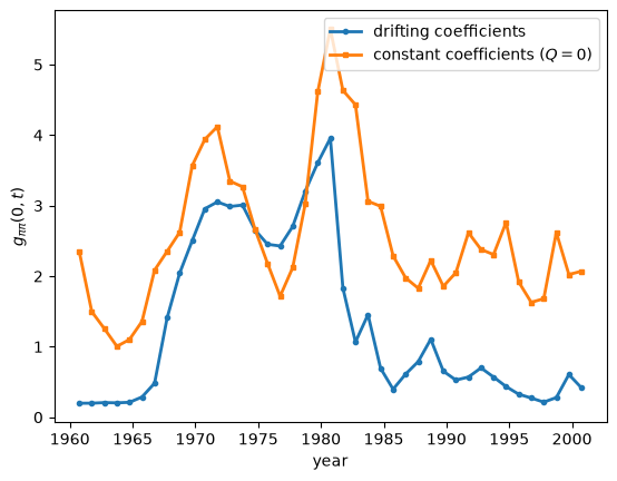
With a fixed \(A\) the persistence measure still moves, because the composition of \(R_t\) — the relative sizes of the three orthogonal shocks — changes even after its overall scale is normalized out.
In fact the constant-coefficient path also climbs to a peak around 1980, as inflation innovations grow large relative to the others, so the bad-luck channel alone can manufacture much of the rise.
What it cannot reproduce is the fall: after 1980 the constant-coefficient persistence stays elevated, around 2 to 3, for the rest of the sample, whereas the drifting-coefficient path collapses back below one.
Freezing \(A\) at its full-sample average leaves inflation propagating almost as strongly in the 1990s as in the 1970s.
So drifting volatility alone accounts for part of the run-up but none of the Volcker-era disinflation of persistence — the post-1980 collapse is evidence about the systematic dynamics, which is exactly why both channels are needed to answer the bad-policy-or-bad-luck question.