92. The Lost Conquest: Fed Policy in the 2020s#
In addition to what’s in Anaconda, this lecture will use the following library to download data from FRED:
!pip install pandas_datareader
92.1. Overview#
This lecture is the contemporary sequel to the Phillips curve tradeoffs suite.
It follows [Sargent and Williams, 2025], which turns the tools of Adaptive Learning and Escape Dynamics and Priors, Escapes, and Learning Cycles — a Phelps control problem, an anticipated-utility government, a drifting-coefficients model estimated by constant-gain recursive least squares, and a self-confirming equilibrium — on the inflation of the 2020s.
The puzzle is a live one.
After the COVID-19 pandemic, U.S. inflation surged to its highest rate since the early 1980s — the very episode we plotted in the post-1999 data of The Rise and Fall of U.S. Inflation.
Yet for more than a year the Federal Reserve did not respond; only in 2022, with inflation already near its peak, did it begin to raise rates aggressively.
Why was the Fed so slow?
[Sargent and Williams, 2025] build an artificial Fed that, each period,
re-estimates a drifting-coefficients Phillips curve by constant-gain recursive least squares, and
solves a linear-quadratic Phelps problem — under an anticipated-utility assumption, in the sense of [Kreps, 1998] — to set its interest-rate instrument.
This is “model predictive control”: the same estimate-then-optimize loop that drove the learning government of Adaptive Learning and Escape Dynamics, but now the instrument is the policy rate and the beliefs concern the persistence of inflation and the slope of the Phillips curve.
Three drifting beliefs turn out to rationalize the slow response:
Declining inflation persistence — the Fed had learned that inflation shocks fade quickly, so the surge looked transitory.
A flatter Phillips curve — the Fed had learned that inflation responds weakly to slack, so disinflation looked costly.
Real-time output-gap mismeasurement — the Fed perceived more economic slack than there really was.
We reproduce the first two from public data, show how they generate a Phelps rule that tracks the actual funds rate, and then — following the paper’s New Keynesian appendix — ask a self-confirming-equilibrium question: were the Fed’s benign beliefs a consequence of its own past success?
Let’s import what we need:
import matplotlib.pyplot as plt
import numpy as np
import pandas as pd
import datetime
from pandas_datareader import data as web
from scipy.linalg import solve_discrete_are
92.2. The three elements#
The first two elements are among the most documented facts in modern macroeconomics.
Declining persistence. From the 1970s into the 1980s inflation was highly persistent; a shock raised inflation for years. [Cogley and Sargent, 2005] and [Stock and Watson, 2007] document a marked decline in persistence after the mid-1980s — inflation began reverting to target much faster.
A flatter Phillips curve. Since the 1990s, estimates of the Phillips curve’s slope have trended toward zero — the “missing disinflation” after the Great Recession being the leading example. Both facts were on policy makers’ minds. Former Fed Chair Janet Yellen observed in 2019 that “the slope of the Phillips curve … has diminished very significantly since the 1960s … and … inflation has become much less persistent.” And, as [Bernanke, 2022] writes, “a flat Phillips curve means that inflation is a less reliable indicator of economic overheating [and] the costs, in terms of unemployment, of bringing inflation back down to target could be higher than in the past.”
Real-time uncertainty. The third element, emphasized by [Orphanides, 2001], is that the output gap is badly mismeasured in real time, especially at business-cycle turning points. Through 2020–2023 the real-time gap was persistently below the later-revised measure, so the Fed perceived more slack — reinforcing the belief that inflation would fade on its own. We use current-vintage data below and return to the real-time distinction in the conclusion.
92.3. The Fed’s drifting-coefficients beliefs#
We give the artificial Fed a backward-looking Phillips curve with drifting coefficients,
where \(\pi_t\) is inflation, \(x_t\) the output gap, \(\rho_t\) the perceived persistence, and \(\kappa_t\) the perceived slope.
The Fed updates \(\theta_t = (\alpha_{0,t}, \rho_t, \kappa_t)\) by constant-gain recursive least squares — exactly the algorithm of Adaptive Learning and Escape Dynamics and Priors, Escapes, and Learning Cycles, with gain \(\gamma\) discounting the past so the estimates can track drift:
with \(X_t = (1, \pi_{t-1}, x_t)'\).
We download quarterly PCE inflation, the CBO output gap, and the federal funds rate from FRED.
start, end = datetime.datetime(1959, 1, 1), datetime.datetime(2025, 7, 1)

pcepi = web.DataReader('PCEPI', 'fred', start, end)['PCEPI'].resample('QS').mean()
gdp   = web.DataReader('GDPC1', 'fred', start, end)['GDPC1']         # real GDP
pot   = web.DataReader('GDPPOT', 'fred', start, end)['GDPPOT']       # CBO potential
ff    = web.DataReader('FEDFUNDS', 'fred', start, end)['FEDFUNDS'].resample('QS').mean()

inflation = 100 * (pcepi / pcepi.shift(4) - 1)     # year-over-year PCE inflation
gap = 100 * (gdp / pot - 1)                        # output gap, percent

data = pd.concat([inflation.rename('pi'), gap.rename('x'),
                  ff.rename('i')], axis=1).dropna()
print(f"sample: {data.index[0].date()} to {data.index[-1].date()}, "
      f"{len(data)} quarters")
sample: 1960-01-01 to 2025-07-01, 263 quarters
Following the paper, we freeze beliefs during 2020–2021 (setting the gain to zero) because the pandemic observations are extreme outliers that would otherwise whipsaw the estimates; belief updating resumes in 2022.
def estimate_beliefs(data, gain=0.03, freeze=(2020, 2021)):
    "Constant-gain RLS of the drifting Phillips curve; returns α₀, ρ, κ paths."
    pi, x = data['pi'].values, data['x'].values
    θ = np.array([0.5, 0.9, 0.05])            # [intercept, persistence, slope]
    R = np.diag([1.0, 10.0, 5.0])
    rows = []
    for t in range(1, len(data)):
        g = 0.0 if data.index[t].year in freeze else gain
        X = np.array([1.0, pi[t - 1], x[t]])
        err = pi[t] - X @ θ
        R = R + g * (np.outer(X, X) - R)
        θ = θ + g * np.linalg.solve(R, X * err)
        rows.append((θ[0], θ[1], θ[2]))
    return pd.DataFrame(rows, index=data.index[1:],
                        columns=['alpha0', 'rho', 'kappa'])

beliefs = estimate_beliefs(data)
fig, axes = plt.subplots(2, 1, figsize=(10, 6), sharex=True)
axes[0].plot(beliefs['rho'])
axes[0].axhline(1, color='k', lw=0.5, ls=':')
axes[0].set_ylabel('persistence $\\rho_t$')
axes[0].set_title('Perceived inflation persistence')

axes[1].plot(beliefs['kappa'], color='C1')
axes[1].axhline(0, color='k', lw=0.5, ls=':')
axes[1].set_ylabel('slope $\\kappa_t$')
axes[1].set_xlabel('year')
axes[1].set_title('Perceived Phillips-curve slope')

plt.tight_layout()
plt.show()
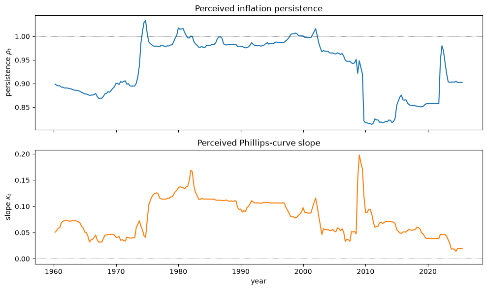
The two panels tell the story.
Perceived persistence \(\rho_t\) is near one through the high-inflation 1970s and 1980s, then drifts down after the mid-1980s, reaching a post-2008 trough — and then jumps back up toward one when belief updating resumes in 2022, just as the Fed abandoned the “transitory” characterization and began to tighten.
Perceived slope \(\kappa_t\) trends toward zero over the 2010s: the Phillips curve flattens.
By 2019 the Fed’s model said inflation was not persistent and only weakly linked to slack — the beliefs that, fed into a Phelps problem, will counsel patience.
92.4. The Fed’s Phelps problem#
Each period the Fed sets its policy rate by solving a linear-quadratic Phelps problem, taking its current estimates as if they will hold forever — the anticipated-utility assumption of [Kreps, 1998] that we met in Adaptive Learning and Escape Dynamics.
Pairing the belief Phillips curve (92.1) with a fixed “IS curve” \(x_t = b_0 + b_1 x_{t-1} + g(i_{t-1} - \pi_{t-1}) + \varepsilon^x_t\) gives linear state dynamics for \(X_t = (1, \pi_t, x_t, i_{t-1})'\),
whose matrices depend on the time-\(t\) beliefs.
The Fed minimizes
where \(\pi^*\) is the 2% target and the last term penalizes abrupt rate changes.
This is a discounted linear-quadratic regulator with a cross-term; its solution is a smoothed Taylor rule \(i_t = -F_t X_t\) whose coefficients move as beliefs move.
# fixed IS curve, estimated once by OLS over the full sample
pi, x, i_ = data['pi'].values, data['x'].values, data['i'].values
n = len(data)
X_is = np.column_stack([np.ones(n - 1), x[:-1], i_[:-1] - pi[:-1]])
b0, b1, g = np.linalg.lstsq(X_is, x[1:], rcond=None)[0]

β, π_star, λ_x, η = 0.95, 2.0, 0.2, 0.5

def phelps_rate(θ, state):
    "Optimal (subjectively) funds rate given beliefs θ=(α₀,ρ,κ) and state."
    α0, ρ, κ = θ
    A = np.array([[1, 0, 0, 0],
                  [α0 + κ * b0, ρ - κ * g, κ * b1, 0],
                  [b0, -g, b1, 0],
                  [0, 0, 0, 0]], float)
    B = np.array([[0], [κ * g], [g], [1]], float)
    c_π = np.array([-π_star, 1, 0, 0.])       # π − π*
    c_x = np.array([0, 0, 1, 0.])             # x
    e_i = np.array([0, 0, 0, 1.])             # i_{-1}
    Q = np.outer(c_π, c_π) + λ_x * np.outer(c_x, c_x) + η * np.outer(e_i, e_i)
    N = (-η * e_i).reshape(4, 1)
    R = np.array([[η]])
    sb = np.sqrt(β)
    P = solve_discrete_are(sb * A, sb * B, Q, R, s=sb * N)
    F = np.linalg.solve(R + β * B.T @ P @ B, β * B.T @ P @ A + N.T)
    return max((-F @ state).item(), 0.0)      # impose the zero lower bound
θ = np.array([0.5, 0.9, 0.05])
R = np.diag([1.0, 10.0, 5.0])
gain = 0.03
opt, θ_2000 = [], None
for t in range(1, n):
    yr = data.index[t].year
    g_t = 0.0 if yr in (2020, 2021) else gain
    X = np.array([1.0, pi[t - 1], x[t]])
    R = R + g_t * (np.outer(X, X) - R)
    θ = θ + g_t * np.linalg.solve(R, X * (pi[t] - X @ θ))
    if data.index[t].year == 2000 and θ_2000 is None:
        θ_2000 = θ.copy()                     # save beliefs for the counterfactual
    state = np.array([1.0, pi[t], x[t], i_[t - 1]])
    opt.append(phelps_rate(θ, state))

optimal = pd.Series(opt, index=data.index[1:])
fig, ax = plt.subplots(figsize=(10, 4.5))
window = slice('1991', None)
ax.plot(optimal[window], 'C0', label="Phelps problem's recommended rate")
ax.plot(data['i'][window], 'C3', lw=1, label='actual federal funds rate')
ax.set_xlabel('year')
ax.set_ylabel('percent')
ax.set_title("The belief-driven Phelps rule vs. actual policy")
ax.legend()
plt.show()

corr = np.corrcoef(optimal['1991':], data['i']['1991':optimal.index[-1]])[0, 1]
print(f"correlation of recommended and actual rate, 1991-2025: {corr:.2f}")
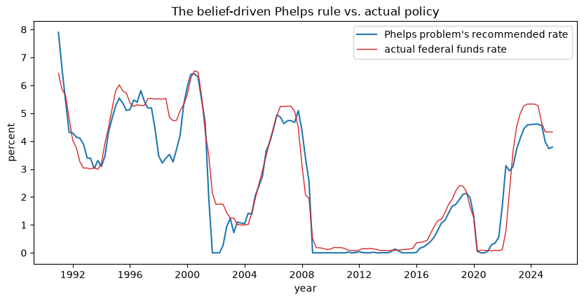
correlation of recommended and actual rate, 1991-2025: 0.95
The subjectively optimal rate tracks the level and turning points of actual policy over three decades (correlation about 0.95): the late-1990s tightening, the 2001 easing, the zero-bound era after 2008, and the 2015 normalization.
Crucially, around the 2021 surge the recommended rate barely moves — the belief-driven rule also counsels a slow response, and only tightens in 2022, mirroring the Fed.
92.5. Why the Fed was slow: a counterfactual#
To isolate the role of the drifting beliefs, we recompute the Phelps recommendations holding beliefs fixed at their January 2000 values — when inflation was still perceived as persistent and the Phillips curve as steeper.
counterfactual = pd.Series(
    [phelps_rate(θ_2000, np.array([1.0, pi[t], x[t], i_[t - 1]]))
     for t in range(1, n)],
    index=data.index[1:])

fig, ax = plt.subplots(figsize=(10, 4.5))
w = slice('2015', None)
ax.plot(optimal[w], 'C0', label='baseline (drifting beliefs)')
ax.plot(counterfactual[w], 'C1--', label='counterfactual (beliefs frozen at 2000)')
ax.plot(data['i'][w], 'C3', lw=1, alpha=0.7, label='actual funds rate')
ax.set_xlabel('year')
ax.set_ylabel('percent')
ax.set_title('Counterfactual: a Fed that had not updated its beliefs since 2000')
ax.legend()
plt.show()
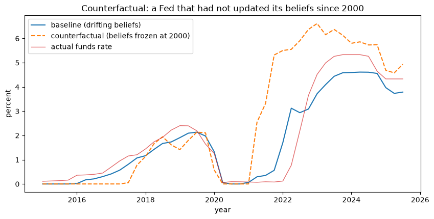
The contrast is stark.
A Fed with year-2000 beliefs — perceiving persistent inflation and a steeper Phillips curve — would have tightened immediately and sharply in 2021, driving the funds rate well above 4% before the actual Fed had moved at all.
The muted, delayed response was not a change in objectives; it was a change in beliefs.
Perceiving inflation as transitory and the Phillips curve as flat, the Fed’s own Phelps problem told it to wait.
92.6. A self-confirming equilibrium: nature’s New Keynesian model#
Were those benign beliefs correct?
Here the paper adds a twist that connects directly to Self-Confirming Equilibria and Escaping Nash Inflation: a self-confirming equilibrium in which the Fed’s flat-Phillips-curve, low-persistence beliefs are a consequence of its own aggressive past policy.
Suppose nature actually runs a small New Keynesian model,
with a structural slope \(\kappa\) and a Taylor rule of aggressiveness \(\phi_\pi\).
In its minimum-state-variable rational expectations equilibrium, \(\mathbb E_t \pi_{t+1} = \lambda\, \pi_t\), where \(\lambda\) — the measured persistence an econometrician would recover — is the stable root of a cubic that depends on \(\phi_\pi\).
The paper proves two comparative statics.
Proposition 92.1 (Aggressive policy lowers measured persistence)
In the determinacy region, the stable root \(\lambda(\phi_\pi)\) is strictly decreasing in the policy aggressiveness \(\phi_\pi\): a more aggressive Fed makes inflation look less persistent.
Proposition 92.2 (Aggressive policy flattens the measured slope)
Under sufficient conditions (a small lagged-inflation term and a sufficiently aggressive rule), the population OLS slope of a backward-looking Phillips curve is also decreasing in \(\phi_\pi\): a more aggressive Fed makes the Phillips curve look flatter.
Let’s reproduce Proposition 92.1 by solving the cubic for the stable root.
def measured_persistence(φ_π, β=0.99, γ_b=0.5, κ=0.1, σ=1.0):
    "Stable MSV root λ(φ_π): the persistence an econometrician would measure."
    coeffs = [β, -(1 + β + κ * σ), 1 + γ_b + κ * σ * φ_π, -γ_b]
    roots = np.roots(coeffs)
    real = roots[np.abs(roots.imag) < 1e-9].real
    stable = real[np.abs(real) < 1.0]
    return stable[np.argmin(np.abs(stable))]

φ_grid = np.linspace(1.05, 3.0, 40)
λ_path = [measured_persistence(φ) for φ in φ_grid]

fig, ax = plt.subplots(figsize=(8, 4.5))
ax.plot(φ_grid, λ_path)
ax.set_xlabel(r'Taylor-rule aggressiveness $\phi_\pi$')
ax.set_ylabel(r'measured persistence $\lambda$')
ax.set_title('Aggressive policy makes inflation look less persistent')
plt.show()
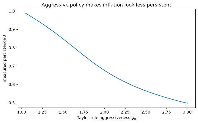
As policy grows more aggressive, the measured persistence falls from near one toward one-half.
The intuition behind both propositions is policy endogeneity, the point emphasized by [McLeay and Tenreyro, 2019]: when the Fed offsets inflationary pressure promptly, a regression that treats the output gap as an exogenous driver recovers a smaller slope and a faster-mean-reverting inflation process than the structural parameters imply.
92.6.1. The trap#
Now read (92.3) as nature and the drifting-coefficients model of the previous sections as the Fed’s approximating model.
Along a path of consistently aggressive policy — the Volcker–Greenspan conquest — the data the Fed generates make inflation look transitory and the Phillips curve look flat.
Estimating its backward-looking model, the Fed comes to believe exactly that.
Those beliefs are a self-confirming equilibrium in the sense of Self-Confirming Equilibria: under the Fed’s current aggressive policy, its reduced-form model is observationally equivalent to nature’s New Keynesian model.
But the beliefs are wrong off the equilibrium path — under a less aggressive policy, persistence and the slope would spring back up.
The Fed cannot see this, because it has no reason to experiment: it sits in the lack-of-experimentation trap of Adaptive Learning and Escape Dynamics, its complacency justified by a belief about a policy it never runs.
When large post-pandemic shocks finally hit, those self-confirming beliefs told the Fed the surge was transitory and tightening was costly — and the conquest was, for a while, lost.
This is a modern replay of the Conquest’s recurrent dynamics, one level up: the mechanism now works through the perceived slope and persistence of the Phillips curve and the policy-rate instrument, and the misspecification is not about expectations but about the policy endogeneity of the reduced-form Phillips curve that the Fed treats as structural — ignoring the Lucas Critique in just the way the “vindication” story of The Rise and Fall of U.S. Inflation describes.
Note
As [Sargent and Williams, 2025] note, the drifting-coefficients model is a purely descriptive “Kepler stage” model, not a structural “Newton stage” one. The paper also acknowledges an alternative reading in which the 2020s accommodation was fiscal in origin — see the fiscal-theory accounts it cites — a very different rationalization of the same policy path.
92.7. Exercises#
Exercise 92.1
The interest-smoothing weight \(\eta\) in the loss (92.2) is, in the paper’s words, “one of the most important parameters.”
Recompute the baseline Phelps recommendations for \(\eta \in \{0.1, 0.5, 2.0\}\) and plot them against the actual funds rate over 2015-2025.
How does a larger smoothing penalty change the character of the recommended policy?
Solution
def recommend(θ_path_fn, η_val):
    global η
    η_save = η
    η = η_val
    θ, R = np.array([0.5, 0.9, 0.05]), np.diag([1.0, 10.0, 5.0])
    out = []
    for t in range(1, n):
        g_t = 0.0 if data.index[t].year in (2020, 2021) else gain
        X = np.array([1.0, pi[t - 1], x[t]])
        R = R + g_t * (np.outer(X, X) - R)
        θ = θ + g_t * np.linalg.solve(R, X * (pi[t] - X @ θ))
        out.append(phelps_rate(θ, np.array([1.0, pi[t], x[t], i_[t - 1]])))
    η = η_save
    return pd.Series(out, index=data.index[1:])

fig, ax = plt.subplots(figsize=(10, 4.5))
w = slice('2015', None)
for η_val in [0.1, 0.5, 2.0]:
    ax.plot(recommend(None, η_val)[w], lw=1, label=rf'$\eta = {η_val}$')
ax.plot(data['i'][w], 'k:', lw=1.5, label='actual')
ax.set_xlabel('year')
ax.set_ylabel('percent')
ax.legend()
plt.show()
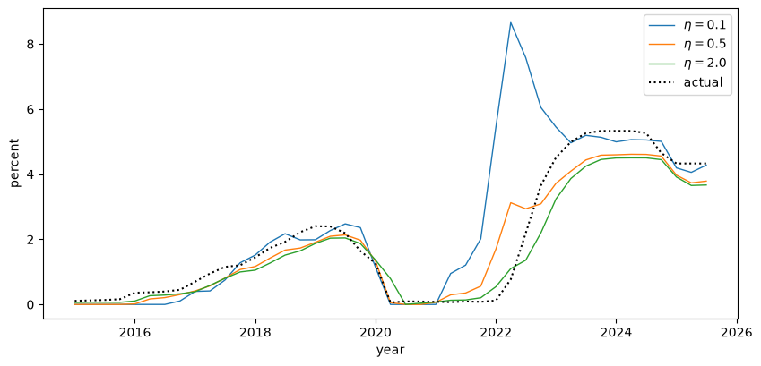
A small \(\eta\) produces a volatile rate that jumps sharply with inflation and the gap; a large \(\eta\) makes the recommendation hug the lagged rate, fitting the smooth observed path better but at the cost of interpretability.
The intermediate value strikes a balance — enough smoothing to resemble real Fed behavior, but still a recognizable response to the state of the economy.
Exercise 92.2
Proposition 92.1 says an aggressive Taylor rule lowers the measured persistence of inflation.
Trace out the implication for the Fed’s own policy by combining the two halves of this lecture: for a grid of structural aggressiveness \(\phi_\pi\), compute the measured persistence \(\lambda(\phi_\pi)\), then feed a belief with that persistence (holding the slope and intercept fixed) into phelps_rate at a representative state, and report the implied inflation response.
Does a Fed that has historically been more aggressive end up less willing to respond to a fresh inflation shock?
Solution
state = np.array([1.0, 4.0, 1.0, 2.0])         # π=4, x=1, i_{-1}=2: an inflation shock

print(f"{'φ_π (history)':>14} {'measured ρ':>12} {'recommended i':>15}")
for φ in [1.2, 1.6, 2.0, 2.6]:
    ρ_meas = measured_persistence(φ)
    i_rec = phelps_rate(np.array([0.3, ρ_meas, 0.05]), state)
    print(f"{φ:>14} {ρ_meas:>12.2f} {i_rec:>15.2f}")
 φ_π (history)   measured ρ   recommended i
           1.2         0.95            3.38
           1.6         0.81            1.85
           2.0         0.68            1.70
           2.6         0.55            1.67
A history of more aggressive policy (higher \(\phi_\pi\)) leaves the Fed believing inflation is less persistent (lower measured \(\rho\)), and — by the logic of Proposition 92.1 together with the comparative statics of the Phelps problem — a Fed that thinks inflation will fade on its own responds less to a fresh shock.
Success breeds complacency: the very aggressiveness that conquered inflation teaches the Fed a lesson that, taken as structural, disarms it against the next surge.