88. Self-Confirming Equilibria#
In addition to what’s in Anaconda, this lecture will use the following library:
!pip install quantecon
88.1. Overview#
This lecture completes the study of Phillips curve tradeoffs begun in The Credibility Problem.
It follows chapter 7 of [Sargent, 1999].
We seek models that depart minimally from the basic [Kydland and Prescott, 1977] model of The Credibility Problem but that also let a government’s beliefs be shaped by the data its own policies generate.
The key equilibrium concept is a self-confirming equilibrium: the government has a possibly wrong model of the Phillips curve, but it fits that model to the data by least squares, and the data it observes confirm its beliefs.
We combine ideas from two literatures:
[King and Watson, 1994] document how inferences about the Phillips curve depend on the direction of fit — whether one regresses unemployment on inflation (a classical identification) or inflation on unemployment (a Keynesian identification).
A literature going back to Muth, Lucas, and Prescott [Lucas and Prescott, 1971, Muth, 1961] formulates rational expectations equilibria as fixed points of mappings from beliefs to the population moments of statistical models.
We build two self-confirming equilibria that are identical except for the direction of fit, and we find that the direction of minimization affects outcomes.
We then study an equilibrium with misspecified beliefs, combining the Phelps problem of Adaptive Expectations and the Phelps Problem with the optimal-misspecification machinery of Optimal Misspecified Beliefs, and find grounds for optimism: outcomes better than Nash, approaching Ramsey as the government becomes patient.
Let’s import what we need:
import matplotlib.pyplot as plt
import numpy as np
import quantecon as qe
from scipy.optimize import minimize_scalar
88.2. Objects in the Phelps problem#
Recall from Adaptive Expectations and the Phelps Problem the ingredients of the general Phelps problem.
The government believes in a reduced-form Phillips curve that it can fit in either direction:
Solving the Phelps problem takes the government’s beliefs \(\gamma\) as given and delivers a decision rule \(h(\gamma)\) for inflation.
The two parameterizations are related by the inversion formulas
88.3. The actual Phillips curve#
The actual Phillips curve extends the one used in earlier lectures to allow for serially correlated shocks:
with \(|\rho_1| < 1\), \(|\rho_2| < 1\), and \(v_t = (v_{1t}, v_{2t})'\) a vector white noise, where \(v_{2t} \equiv y_t - x_t\) is the surprise in inflation.
For much of this lecture we set \(\rho_1 = \rho_2 = 0\) to make theoretical points, which reduces (88.2) to
88.4. Self-confirming equilibria#
A self-confirming equilibrium reconciles the government’s beliefs with the environment those beliefs generate.
Definition 88.1 (Self-confirming equilibrium)
A self-confirming equilibrium is a fixed belief vector \(\gamma\), a government decision rule \(h = h(\gamma)\), and a stationary process for \((y_t, U_t, x_t)\) such that
(a) inflation solves the Phelps problem, \(y_t = h X_{t-1} + v_{2t}\);
(b) the public optimally forecasts inflation, \(x_t = h X_{t-1}\);
© unemployment is generated by the actual Phillips curve (88.2); and
(d) the government’s beliefs satisfy the least squares orthogonality conditions \(E\left[U_t - \gamma' X_{C,t}\right] X_{C,t}' = 0\) (the classical direction of fit).
Condition (d) makes the government’s beliefs depend on moment matrices that, through (a)–©, themselves depend on the government’s beliefs.
The government’s beliefs imply behavior that produces data whose moments confirm those beliefs.
A distinct self-confirming equilibrium results from replacing (d) with the Keynesian direction of fit:
(d′) the government fits the Keynesian Phillips curve, \(E\left[y_t - \beta' X_{K,t}\right] X_{K,t}' = 0\), then recovers \(\gamma\) from the inversion formulas (88.1).
Because the government’s beliefs affect the whole probability distribution of the data, the direction of minimization affects outcomes.
Note
Computing a self-confirming equilibrium in general means finding a fixed point of a map \(\gamma = T(h(\gamma))\) (classical) or \(\beta = S(h(\gamma(\beta)))\) (Keynesian). The moments in the orthogonality conditions are obtained from the state-space representation of the system by solving a discrete Lyapunov equation. In practice one iterates a relaxation algorithm \(\beta_{j+1} = \kappa\beta_j + (1-\kappa) S(\beta_j)\), which resembles the least squares learning recursion of The Credibility Problem.
88.5. The special case solved by hand#
When \(\rho_1 = \rho_2 = 0\), the government’s problem collapses to a sequence of static problems, and each self-confirming equilibrium can be computed by hand.
With \(X_{t-1} = 1\), the actual Phillips curve implies the second moments
Classical direction of fit (\(U\) on \(y\)): the slope is
and the requirement that the means lie on the regression line gives the intercept \(\gamma_{-1} = (\gamma_1^2 + 1) U^*\).
Keynesian direction of fit (\(y\) on \(U\)): the slope is
with intercept \(\beta_{-1} = -\frac{\beta_1^2 + 1}{\beta_1} U^*\), from which the implied classical coefficients follow by inversion, \(\gamma_1 = \beta_1^{-1}\) and \(\gamma_{-1} = \frac{\beta_1^2 + 1}{\beta_1^2} U^*\).
class SelfConfirmingStatic:
    """
    The two static self-confirming equilibria (ρ1 = ρ2 = 0), one for
    each direction of fit.
    """

    def __init__(self, θ=1.0, U_star=5.0, σ1=0.3, σ2=0.3):
        self.θ, self.U_star, self.σ1, self.σ2 = θ, U_star, σ1, σ2

    def classical(self):
        "Perceived Phillips curve U = γ_{-1} + γ_1 y under classical fit."
        θ, U_star = self.θ, self.U_star
        γ1 = -θ
        γ_1 = (γ1**2 + 1) * U_star
        y_bar = -γ_1 * γ1 / (γ1**2 + 1)      # mean (= Nash) inflation
        return γ1, γ_1, y_bar

    def keynesian(self):
        "Perceived Phillips curve under Keynesian fit, inverted to γ."
        θ, U_star, σ1, σ2 = self.θ, self.U_star, self.σ1, self.σ2
        β1 = -θ * σ2**2 / (σ1**2 + θ**2 * σ2**2)
        β_1 = -(β1**2 + 1) / β1 * U_star
        γ1 = 1 / β1
        γ_1 = (β1**2 + 1) / β1**2 * U_star
        y_bar = β_1 / (β1**2 + 1)             # mean inflation
        return γ1, γ_1, y_bar
sce = SelfConfirmingStatic(θ=1.0, U_star=5.0, σ1=0.3, σ2=0.3)

γ1_C, γ0_C, y_C = sce.classical()
γ1_K, γ0_K, y_K = sce.keynesian()

print("Classical direction of fit")
print(f"  γ_1 = {γ1_C:.1f},  γ_(-1) = {γ0_C:.1f},  mean inflation = {y_C:.1f}")
print("Keynesian direction of fit")
print(f"  γ_1 = {γ1_K:.1f},  γ_(-1) = {γ0_K:.1f},  mean inflation = {y_K:.1f}")
Classical direction of fit
  γ_1 = -1.0,  γ_(-1) = 10.0,  mean inflation = 5.0
Keynesian direction of fit
  γ_1 = -2.0,  γ_(-1) = 25.0,  mean inflation = 10.0
These reproduce the numerical example of chapter 7 of [Sargent, 1999].
Under the classical direction of fit, mean inflation is the Nash value \(\theta U^* = 5\).
Under the Keynesian direction of fit, the government estimates a flatter Phillips curve and believes the tradeoff is more favorable than it is, so it sets inflation twice as high, at \(10\).
Let’s draw the two self-confirming Phillips curves, reproducing Figure 7.1.
fig, ax = plt.subplots(figsize=(7, 6))

U_grid = np.linspace(0, 12, 100)

# perceived Phillips curves U = γ_{-1} + γ_1 y  =>  y = (U - γ_{-1}) / γ_1
ax.plot(U_grid, (U_grid - γ0_C) / γ1_C, 'C0', label='P: classical fit')
ax.plot(U_grid, (U_grid - γ0_K) / γ1_K, 'C1', label='Q: Keynesian fit')

ax.plot(sce.U_star, y_C, 'C0o')
ax.annotate('Nash', (sce.U_star, y_C), (sce.U_star + 0.4, y_C - 0.6))
ax.plot(sce.U_star, y_K, 'C1o')
ax.annotate('Keynesian mean', (sce.U_star, y_K),
            (sce.U_star + 0.4, y_K + 0.2))

ax.set_xlim(0, 12)
ax.set_ylim(0, 12)
ax.set_xlabel('unemployment $U$')
ax.set_ylabel('inflation $y$')
ax.legend()
plt.show()
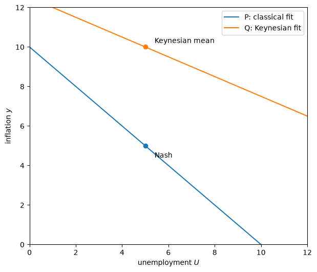
Curve P is the self-confirming Phillips curve estimated with the classical direction of fit; curve Q with the Keynesian direction.
Because the Keynesian fit makes the government believe the tradeoff is more exploitable, average inflation is higher.
88.5.1. Why not Ramsey?#
Both self-confirming equilibria give a mean outcome worse than the Ramsey outcome.
This signifies a breakdown of the hypotheses of the proposition in Adaptive Expectations and the Phelps Problem that solving the Phelps problem eventually sustains nearly the Ramsey outcome.
What fails is the induction hypothesis.
Because \(\rho_1 = \rho_2 = 0\), the self-confirming equilibria are serially uncorrelated, so lagged inflation drops out of the empirical Phillips curves.
Deactivating the induction hypothesis makes the government in effect solve a one-period problem and shuts down the intertemporal channel that promotes better outcomes.
88.6. Equilibrium with misspecified beliefs#
To explore how imputing a different wrong model might improve on the Nash outcome, we now let the public, not the government, make a subtle specification error.
This links adaptive expectations, the induction hypothesis, and the Phelps problem.
The government knows the correct model,
where the public has constant-gain adaptive expectations with a parameter \(C\) that it tunes to fit the data.
Taking \(x_t\) as a state variable, the government solves the Phelps problem: it maximizes \(-E_0 \sum_{t=0}^\infty \delta^t\left[(U^* - \theta(y_t - x_t))^2 + y_t^2\right]\) by choice of a feedback rule \(y_t = f_1 + f_2 x_t + v_{2t}\).
This is exactly the LQ Phelps problem of Adaptive Expectations and the Phelps Problem with adaptation parameter \(\lambda = 1 - C\).
def phelps_policy(C, δ, θ=1.0, U_star=5.0):
    "Government feedback rule y_t = f1 + f2 x_t, with public gain C."
    λ = 1 - C
    a = np.array([[U_star], [θ]])
    R = 0.5 * (a @ a.T)
    Q = np.array([[0.5 * (θ**2 + 1)]])
    N = -0.5 * θ * a.T
    A = np.array([[1.0, 0.0], [0.0, λ]])
    B = np.array([[0.0], [1 - λ]])
    lq = qe.LQ(Q, R, A, B, N=N, beta=min(δ, 1 - 1e-7))
    P, F, d = lq.stationary_values()
    return -F[0, 0], -F[0, 1]
The government’s behavior makes the actual inflation rate
with mean \(\nu = f_1 / (1 - f_2)\) and spectrum \(F(\omega; C) = |f(e^{i\omega})|^2 \sigma_2^2\).
Given \(C\), the public seeks the best-fitting misspecified model of the same integrated moving-average form as in Optimal Misspecified Beliefs,
and the induced best-estimate map \(c = B(C)\) defines an equilibrium under forecast misspecification as a fixed point \(C = B(C)\).
This makes both the true and the approximating models equilibrium outcomes, and turns the adaptation parameter \(C\) into an outcome rather than a free parameter.
class MisspecifiedPhillips:
    """
    Equilibrium with misspecified public beliefs: a fixed point of the
    best-estimate map, with the government solving the Phelps problem.
    """

    def __init__(self, θ=1.0, U_star=5.0, σ2=0.3, δ=0.97, ρ=0.995, N=1024):
        self.θ, self.U_star, self.σ2 = θ, U_star, σ2
        self.δ, self.ρ, self.N = δ, ρ, N
        ω = 2 * np.pi * np.arange(N) / N
        self.z = np.exp(1j * ω)
        self.ω = ω

    def true_process(self, C):
        "Return the mean ν, spectrum F, and policy (f1, f2) given belief C."
        f1, f2 = phelps_policy(C, self.δ, self.θ, self.U_star)
        ν = f1 / (1 - f2)
        ψ = 1 - C * (1 - f2)
        f = (1 - (1 - C) * self.z) / (1 - ψ * self.z)
        F = np.abs(f)**2 * self.σ2**2
        return ν, F, (f1, f2)

    def best_estimate(self, C):
        "The best-estimate map c = B(C)."
        ν, F, _ = self.true_process(C)
        z, ρ = self.z, self.ρ

        def profile(c):
            H = np.abs((1 - (1 - c) * z) / (1 - ρ * z))**2
            σ_ε2 = np.mean(F / H) + ν**2 / H[0]
            return np.log(σ_ε2) + np.mean(np.log(H))

        return minimize_scalar(profile, bounds=(1e-4, 0.99),
                               method='bounded').x

    def solve(self, C0=0.1, tol=1e-10, maxit=500):
        "Iterate the best-estimate map to a fixed point."
        C = C0
        for _ in range(maxit):
            C_new = self.best_estimate(C)
            if abs(C_new - C) < tol:
                break
            C = C_new
        ν, _, (f1, f2) = self.true_process(C_new)
        return C_new, ν, (f1, f2)
mp = MisspecifiedPhillips(δ=0.97)
C_star, ν_star, (f1, f2) = mp.solve()

print(f"equilibrium gain     C = {C_star:.4f}")
print(f"policy rule          y = {f1:.4f} + {f2:.4f} x")
print(f"mean inflation       ν = {ν_star:.3f}")
print(f"Nash inflation   θ U*  = {mp.θ * mp.U_star:.3f}")
equilibrium gain     C = 0.1138
policy rule          y = 0.7109 + 0.3348 x
mean inflation       ν = 1.069
Nash inflation   θ U*  = 5.000
The most important outcome is that the implied mean inflation rate is substantially below the Nash value of \(5\).
The induction hypothesis embedded in the adaptive expectations scheme, together with a high discount factor, delivers this improvement — and because \(C\) is now an equilibrium outcome, the mechanism is sharper than in Adaptive Expectations and the Phelps Problem, where \(C\) could be manipulated independently of \(\delta\).
88.6.1. Approaching Ramsey#
As the government becomes more patient, the equilibrium mean inflation rate falls toward the Ramsey value of zero.
δ_grid = np.array([0.95, 0.96, 0.97, 0.98, 0.99, 0.995])
C_vals, ν_vals = [], []
for δ in δ_grid:
    C, ν, _ = MisspecifiedPhillips(δ=δ).solve()
    C_vals.append(C)
    ν_vals.append(ν)

fig, axes = plt.subplots(1, 2, figsize=(11, 4.5))
axes[0].plot(δ_grid, ν_vals, 'o-')
axes[0].axhline(mp.θ * mp.U_star, color='k', ls='--', lw=1, label='Nash')
axes[0].set_xlabel(r'discount factor $\delta$')
axes[0].set_ylabel('mean inflation')
axes[0].legend()

axes[1].plot(δ_grid, C_vals, 'o-', color='C1')
axes[1].set_xlabel(r'discount factor $\delta$')
axes[1].set_ylabel('equilibrium gain $C$')

plt.tight_layout()
plt.show()
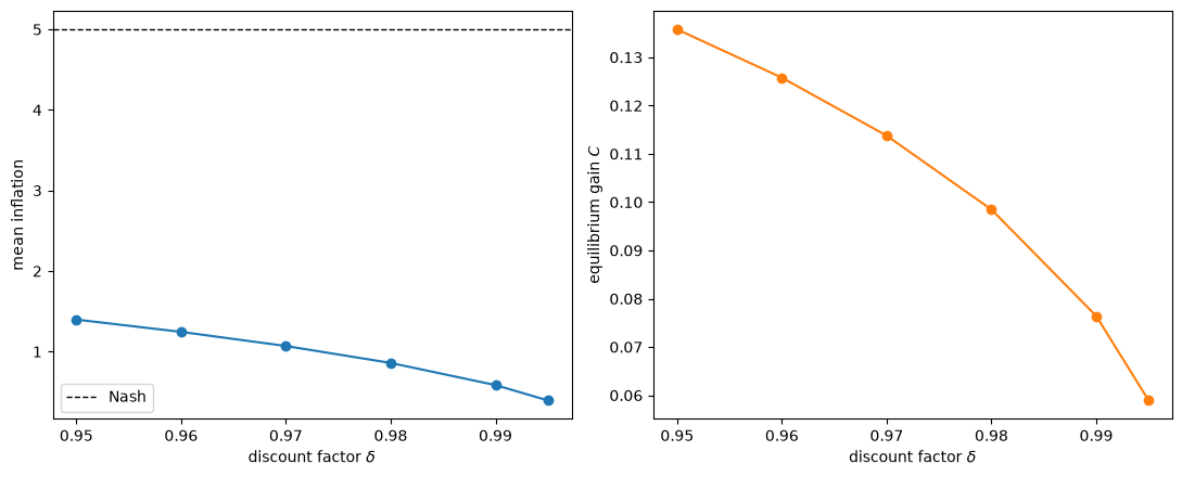
Mean inflation lies far below the Nash value at every discount factor and declines toward the Ramsey value of zero as \(\delta \to 1\).
Note
The precise equilibrium values depend on the near–unit-root approximation \(\rho\) used to keep the perceived model’s spectral density well defined, as discussed in Optimal Misspecified Beliefs. The qualitative conclusion — better-than-Nash outcomes that approach Ramsey as \(\delta \to 1\) — is robust.
88.6.2. Spectra and impulse responses#
Let’s compare the true and approximating inflation processes at the equilibrium, as in Figures 7.2 and 7.3 of [Sargent, 1999].
ν_star, F, _ = mp.true_process(C_star)
c_star = mp.best_estimate(C_star)
H = np.abs((1 - (1 - c_star) * mp.z) / (1 - mp.ρ * mp.z))**2
σ_ε2 = np.mean(F / H) + ν_star**2 / H[0]
G = H * σ_ε2

half = mp.N // 2
fig, ax = plt.subplots(figsize=(8, 5))
ax.plot(mp.ω[:half], np.log(F[:half]), 'C0', label='true model')
ax.plot(mp.ω[:half], np.log(G[:half]), 'C1--', label='approximating model')
ax.set_xlabel(r'angular frequency $\omega$')
ax.set_ylabel('log spectral density')
ax.legend()
plt.show()
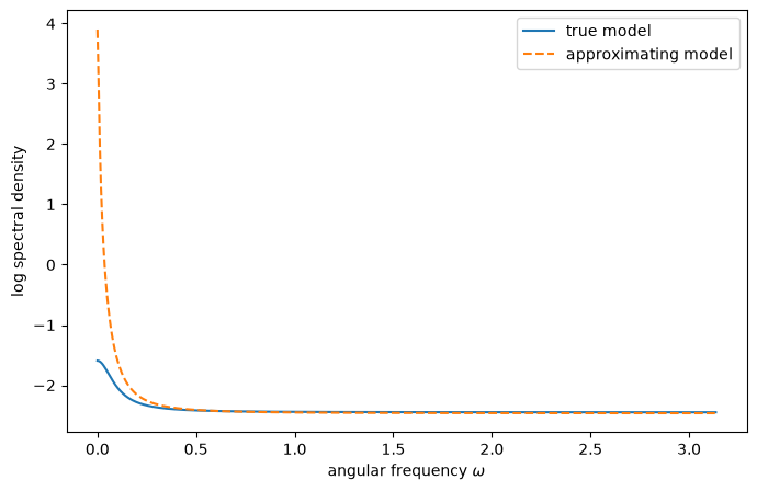
The true and approximating spectral densities match well at all but the lowest frequencies.
The true inflation rate is only moderately serially correlated, and — as in the Bray model of Optimal Misspecified Beliefs — the approximating model uses a unit root to simulate a mean, capturing first moments with second moments.
def ima_impulse(num, den, T=25):
    "IRF of (1 - num L)/(1 - den L)."
    h = np.empty(T)
    h[0] = 1.0
    for k in range(1, T):
        h[k] = den * h[k - 1]
    h[1:] -= num * h[:-1]
    return h

ψ = 1 - C_star * (1 - f2)
irf_true = ima_impulse(1 - C_star, ψ)
irf_approx = ima_impulse(1 - c_star, mp.ρ)

fig, ax = plt.subplots(figsize=(8, 5))
ax.plot(irf_true, 'C0o-', ms=4, label='true model')
ax.plot(irf_approx, 'C1s--', ms=4, label='approximating model')
ax.set_xlabel('lag')
ax.set_ylabel('response')
ax.legend()
plt.show()
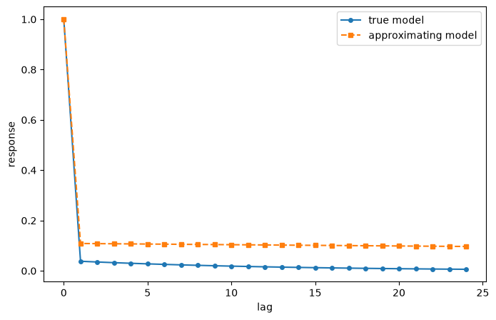
The unit root in the approximating model manifests itself as a nonzero asymptote in its impulse response.
88.6.3. Grounds for optimism#
After the disappointments of the self-confirming equilibria, the equilibrium with forecast misspecification is heartening: it supports better-than-Nash outcomes.
The equilibrium concept is not self-confirming, but it has that spirit — it embodies a type of self-confirmation with a wrong model.
That the approximation error is small shows there is a nearly self-confirming model with much better than Nash outcomes.
The next lectures in this suite — Adaptive Learning and Escape Dynamics, Escaping Nash Inflation, and Priors, Escapes, and Learning Cycles — build adaptive, real-time versions of these models in which the government estimates its Phillips curve recursively from the most recent data.
There the self-confirming equilibrium computed here becomes the attractor of the learning dynamics, and the better-than-Nash outcomes reappear as recurrent escapes away from it.
88.7. Exercises#
Exercise 88.1
The gap between the two static self-confirming equilibria is driven by the variances \(\sigma_1\) (the Phillips curve shock) and \(\sigma_2\) (the inflation surprise).
The classical equilibrium always delivers mean inflation equal to the Nash value \(\theta U^*\), but the Keynesian mean inflation depends on the ratio \(\sigma_1 / \sigma_2\).
Fixing \(\sigma_2 = 0.3\), \(\theta = 1\), \(U^* = 5\), plot Keynesian mean inflation as a function of \(\sigma_1 \in [0.05, 1.0]\).
What happens as \(\sigma_1 \to 0\), and why?
Solution
σ1_grid = np.linspace(0.05, 1.0, 50)
y_keynes = [SelfConfirmingStatic(σ1=σ1, σ2=0.3).keynesian()[2]
            for σ1 in σ1_grid]

fig, ax = plt.subplots(figsize=(8, 4.5))
ax.plot(σ1_grid, y_keynes, label='Keynesian mean inflation')
ax.axhline(5.0, color='k', ls='--', lw=1, label='Nash')
ax.set_xlabel(r'$\sigma_1$')
ax.set_ylabel('mean inflation')
ax.legend()
plt.show()
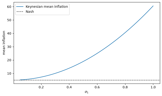
As \(\sigma_1 \to 0\) the Phillips curve becomes nearly deterministic, the Keynesian slope \(\beta_1 \to -1/\theta\), and the two directions of fit agree, so Keynesian mean inflation approaches the Nash value.
As \(\sigma_1\) grows, unemployment becomes noisier, the Keynesian regression of \(y\) on \(U\) flattens, and the government perceives a more exploitable tradeoff, raising mean inflation.
Exercise 88.2
Verify that the misspecified-beliefs equilibrium is a genuine fixed point.
For \(\delta = 0.97\), plot the best-estimate map \(C \mapsto B(C)\) against the 45-degree line and mark the fixed point.
Solution
mp = MisspecifiedPhillips(δ=0.97)
C_grid = np.linspace(0.02, 0.3, 20)
B_vals = [mp.best_estimate(C) for C in C_grid]
C_star, _, _ = mp.solve()

fig, ax = plt.subplots(figsize=(6, 6))
ax.plot(C_grid, B_vals, 'C0', label='$B(C)$')
ax.plot(C_grid, C_grid, 'k--', lw=1, label='45 degrees')
ax.plot(C_star, C_star, 'ko')
ax.annotate('equilibrium', (C_star, C_star), (C_star + 0.03, C_star - 0.03))
ax.set_xlabel('$C$')
ax.set_ylabel('$B(C)$')
ax.legend()
plt.show()
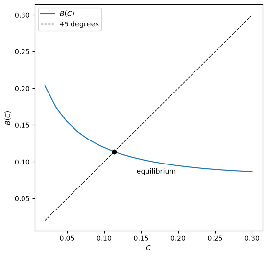
The best-estimate map crosses the 45-degree line at the equilibrium gain, confirming \(C = B(C)\).